
Type a question into a chat box and an answer streams back. Between those two moments sits a fixed, knowable sequence of operations. LLM inference is not a black box. It is about a dozen stages, and every one of them can be named, measured, and reasoned about with arithmetic you can do on paper.
This article traces one prompt end to end: "What is a quadratic equation?". The model is a Llama-3-70B class model. 80 layers, d_model 8,192, 64 query heads, 8 key/value heads, head_dim 128, FFN width 28,672, vocabulary 128,256, roughly 140 GB of bf16 weights. The numbers belong to that model. The structure belongs to every decoder-only transformer running in production today.
By the end you will be able to point at any stage of LLM inference and say what it reads, what it writes, what it costs, and whether it is limited by arithmetic or by memory bandwidth. That last distinction is the one that sets your GPU bill.
- Part 1. How an LLM Answers a Question: The Complete Inference Path (you are here)
- Part 2. Byte-Pair Encoding Explained: How LLMs Turn Text Into Tokens
- Part 3. Inside One Transformer Block: The Residual Stream and Its Seven Matrices
- Part 4. Multi-Head Attention Explained: Why 64 Heads Instead of One
- Part 5. The Output Projection: How 64 Attention Heads Become One Thought
- Part 6. The Feed-Forward Network: Where a Transformer Keeps What It Knows
- Part 7. Mixture of Experts Explained: Conditional Computation From Zero
- Part 8. Attention Is All You Need, Dissected: The 2017 Figure, Box by Box
- Part 9. The Roofline Model: Why LLM Decode Is Memory-Bound
- Part 10. Continuous Batching and PagedAttention: How vLLM Keeps a GPU Busy
- Part 11. Benchmark Your Own LLM Serving Stack: Two Measurements, One Afternoon
How to read this series
This is Part 1 of eleven. It is the map. Every later part takes one box on this map and opens it. You can read them in order, or land here, find the stage you care about, and jump.

| Part | Title | What you get |
|---|---|---|
| 1 | How an LLM Answers a Question: The Complete Inference Path (you are here) | The whole path, every stage named and costed. |
| 2 | Byte-Pair Encoding Explained: How LLMs Turn Text Into Tokens | How the merge list is built, and why “quadratic” costs two tokens. |
| 3 | Inside One Transformer Block: The Residual Stream and Its Seven Matrices | One block end to end, in the order the operations run. |
| 4 | Multi-Head Attention Explained: Why 64 Heads Instead of One | What a head is, and what splitting buys that one big attention cannot. |
| 5 | The Output Projection: How 64 Attention Heads Become One Thought | What W_O does, and why concatenation alone is not enough. |
| 6 | The Feed-Forward Network: Where a Transformer Keeps What It Knows | The 82 percent of each layer that most explanations skip. |
| 7 | Mixture of Experts Explained: Conditional Computation From Zero | Replacing one feed-forward network with many, plus a router. |
| 8 | Attention Is All You Need, Dissected: The 2017 Figure, Box by Box | The original diagram read against a model that shipped last year. |
| 9 | The Roofline Model: Why LLM Decode Is Memory-Bound | Arithmetic intensity, the balance point, and where each stage lands. |
| 10 | Continuous Batching and PagedAttention: How vLLM Keeps a GPU Busy | How a real server keeps the batch full and the cache unfragmented. |
| 11 | Benchmark Your Own LLM Serving Stack: Two Measurements, One Afternoon | Two numbers you can measure today that predict everything else. |
The route, before the detail
Orientation first. There are two neural phases separated by one non-neural decision, and the whole thing is wrapped in a tokenizer that is not a neural network at all.
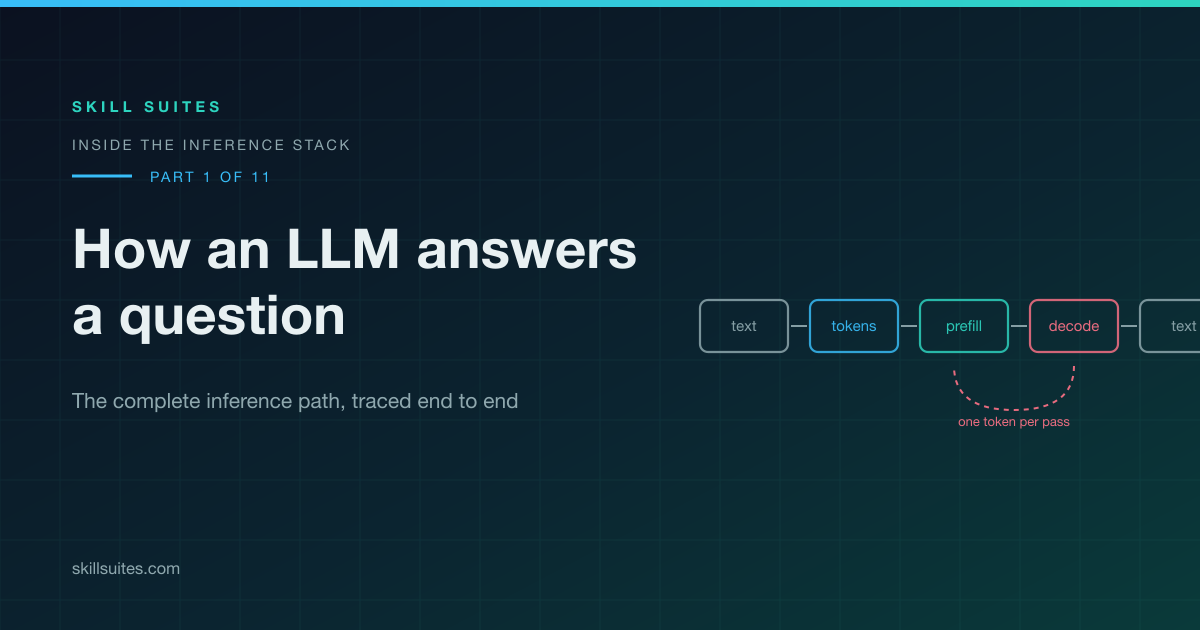
Prefill reads the prompt. Sampling picks a token. Decode produces every remaining token, one full pass through the model per token, until the model emits a stop token. Everything below is detail hanging off those five boxes.
Stage 0: a trained model is a directory of numbers
There is no code inside a trained model. No rules, no logic, no branches. There are about 70 billion floating-point values arranged into named arrays, and a small generic program that multiplies them together in a fixed order. All of the behaviour lives in the numbers.
Those numbers are grouped into 80 layers of identical structure. Layer 1 and layer 80 have the same shapes and run the same operations, and only the values differ. That repetition is why one description of a layer describes the whole model, and why the middle of this article spends its length on one layer and then says “now do that 79 more times”.
At bf16, two bytes per value, the directory is roughly 140 GB: a 2.1 GB embedding table, 80 layers at 1.712 GB each, and a 2.1 GB output projection at the end.
Keep one distinction straight from here on. Weights are the model: fixed, shared by every user, identical for every prompt, 140 GB. Activations are the numbers flowing through for one particular request: different every time, discarded immediately, measured in kilobytes. Nearly every confusion about LLM memory comes from mixing the two. The KV cache is the single exception, the activations that are deliberately kept.
Stage 1: characters become integers
Nothing neural has happened yet. A separate piece of software, the tokenizer, converts your string into a list of integers by replaying a merge list learned from a corpus. No gradients, no network, no learning at runtime.
"What is a quadratic equation?" becomes seven integers. Notice what happens to the word “quadratic”. It is not in the vocabulary, so it arrives in two pieces, and the model will never know it was one word. The leading space is part of the token too, which is why " is" and "is" are separate vocabulary entries.
From this point the model has no access to letters. Every question you have ever asked it about spelling, character counting, or rhyme was answered by something that cannot see characters. Part 2 builds this vocabulary from scratch, including why non-English text often costs two or three times more tokens for the same content.
Stage 2: integers become vectors, and gain a position
Each of the seven IDs is used as a row index into the embedding table, a matrix of 128,256 rows and 8,192 columns. Row 30236 is copied out and becomes the starting vector for quad. This is a lookup, not a multiplication. No arithmetic runs. A row is copied.
After this step the prompt is seven vectors of 8,192 numbers, about 229 KB of activations drawn from 2.1 GB of table, and the integers have done their only job. No single number in those 8,192 means anything on its own. Properties are encoded as directions across many numbers at once, which is why you cannot inspect a model by reading its embeddings.
Position, injected by rotation
Attention compares tokens using dot products, and a dot product has no idea where its operands came from. With no intervention, “What is a quadratic equation” and “equation quadratic a is What” produce identical numbers. A transformer is a bag of words until position is forced into the vectors.
Llama does it by rotating. Read a 128-number head vector as 64 pairs, treat each pair as a point on a plane, and rotate each pair by an angle proportional to the token’s position in the sequence, 0, 1, 2, 3. Not its ID. This is RoPE. It touches queries and keys only, and it has zero learned parameters.
Rotation beats addition for an algebraic reason. Rotate the query by position m and the key by position n, then dot them, and the absolute positions cancel. Only the gap n minus m survives. The model never learns “position 47”. It learns “three tokens back”, which is the thing that generalises to position 4,700.
Stage 3: inside one layer
This is the substance of the model. Ten operations run in a fixed order, and then the whole thing repeats 79 more times with different numbers.
Hold two facts before the detail. First, only one of the ten operations lets a token see another token, and that is attention. The other nine process each position in complete isolation. Second, the layer does not replace its input. It computes an adjustment and adds it. What flows from layer to layer is a running total, which is what makes 80 layers trainable at all and why the vector width never changes.
Where the weights actually are
Here is the correction most mental models need. Attention is one of five weight-bearing operations in a layer, and it is not the expensive one.
| Matrix | Shape | Bytes at bf16 | Group |
|---|---|---|---|
W_Q |
8192 by 8192 | 134 MB | attention |
W_K |
8192 by 1024 | 17 MB | attention |
W_V |
8192 by 1024 | 17 MB | attention |
W_O |
8192 by 8192 | 134 MB | attention |
W_gate |
8192 by 28672 | 470 MB | FFN |
W_up |
8192 by 28672 | 470 MB | FFN |
W_down |
28672 by 8192 | 470 MB | FFN |
| 2 RMSNorm gain vectors | 8192 each | 32 KB | norm |
| attention subtotal | 302 MB | 18 percent | |
| FFN subtotal | 1,410 MB | 82 percent | |
| one layer | 1,712 MB | ||
| 80 layers | 137 GB | read on every forward pass |
The feed-forward network holds 82 percent of the layer’s parameters. Attention gets the conceptual spotlight. The MLP holds the numbers. “It uses attention to check the words” describes one step out of five, and the other four know nothing about your question at all. They are the model itself.
Query, key, and value, and why there are only eight K/V heads
The normalised vector is multiplied by three separate learned matrices, producing three views of the same token. Query is what this token is searching for. Key is what it advertises about itself. Value is what it hands over on a match. The names come from database lookup and have nothing to do with your prompt happening to be a question.
Watch the shapes. Q comes out 8,192 wide, K and V come out 1,024 wide. That asymmetry is grouped-query attention: 64 query heads divided into 8 groups, with every query in a group reading the same key and value head. Queries stay diverse. The material being searched is shared eight ways.
The reason is cache size, because K and V are stored for later while Q is discarded the moment it is used. With 8 K/V heads this model spends 0.33 MB of cache per token. With a full 64 it would spend 2.5 MB, and one user with an 8,000-token conversation would need 20 GB to themselves. Part 4 takes the head split apart properly.
Attention: the only step where tokens see each other
Take this token’s query. Dot it against every cached key to get one similarity score per position. Divide by the square root of 128. Blank out anything in the future. Softmax the scores into probabilities. Use those probabilities to take a weighted average of the value vectors. Run all of that 64 times independently, then concatenate.
The division is not a tuning knob. Softmax exponentiates, so unscaled scores of 128 summed terms would collapse the distribution onto a single token. Dividing by the square root of head_dim restores about unit variance and keeps the distribution soft.
Then W_O, another 8192 by 8192 matrix, mixes the 64 heads’ independent findings into one coherent update. Without it, head 12’s discovery could never inform head 40’s, and multi-head attention would be 64 parallel operations rather than one.
The triangle is what makes the KV cache legal
Every score for a future position is set to negative infinity before softmax, which becomes exactly zero after exponentiation. Position 0 attends only to itself. Position 6 attends to all seven. The result is a lower triangle.
That restriction is worth more than the mask itself. Because nothing later can influence an earlier token, that token’s key and value are final the moment they are computed. They can be written once and reused for every subsequent step, forever. Remove the mask, as encoder models like BERT do, and every token’s representation changes when new tokens arrive. No cache is possible, and generation as a loop is not possible either.
The size formula is worth memorising: bytes = 2 x layers x kv_heads x head_dim x tokens x dtype_bytes. For this model that is 2 x 80 x 8 x 128 x 2 = 327,680 bytes per token. A seven-token prompt occupies 2.3 MB. An 8,000-token conversation occupies 2.6 GB, for one user. Weights amortise across everybody on the GPU. Cache does not, which is why reusing a shared prompt prefix changes the economics so sharply.
The feed-forward network, where the parameters live
Expand 8,192 to 28,672 twice in parallel. Pass one branch through SiLU and use it to gate the other, elementwise. Compress back to 8,192. Three matrices, one nonlinearity, one elementwise multiply. This is SwiGLU.
Two things matter here. The nonlinearity is mandatory: two matrix multiplies in sequence equal a single matrix multiply, so 80 layers of pure linear algebra would be exactly as expressive as one. And the block operates on each token alone. Position 3 and position 6 never interact anywhere inside it. Attention gathered information from elsewhere; the FFN is where the model works on it privately, and where model-editing research consistently finds facts stored. Part 6 is entirely about this block.
Stage 4: prefill, all seven tokens in one pass
Now run everything above 80 times. Layer 1’s output vectors become layer 2’s inputs, and layer 2 has its own completely separate 1.712 GB. No weights are shared between layers.
The seven tokens travel together. Each weight matrix is loaded from memory once and used for all seven simultaneously: one matrix multiply with seven rows instead of seven separate multiplies. That single fact is the entire difference between this phase and the next one.
The number to watch is arithmetic intensity, meaning FLOPs performed per byte moved from memory. Reading 137 GB of weights to serve seven tokens gives roughly 2 x 7 = 14 FLOPs per byte. An H100 needs about 295 to keep its arithmetic units fed, so a seven-token prompt does not get there. A realistic 2,000-token prompt reaches roughly 4,000 and is comfortably compute-bound. Prompt length is what moves this stage, not the model.
By layer 80 the cache holds 7 positions across 80 layers: 2.3 MB, against the 137 GB of weights just read. The elapsed time here is your time to first token, which is the number streaming is designed to hide.
Stage 5: six of seven outputs are discarded
After layer 80 you hold seven output vectors, one per input token. Six are thrown away. Only the vector at the final position, the one belonging to ?, is used, because the causal mask means only that position has attended to the entire prompt.
During training all seven would be used, each predicting its own next token, which is how one document becomes thousands of simultaneous training examples. At inference the other six existed purely to give the last one context.
The surviving vector meets the LM head, an 8,192 by 128,256 matrix, and comes out as 128,256 logits: one raw, unnormalised score per vocabulary entry.
Stage 6: sampling, the only randomness in the system
The model never chooses a token. It produces a distribution, and a separate, non-neural step draws from it. That step is entirely under your control, and it is the only place randomness enters LLM inference at all.
Softmax converts logits into probabilities. Three knobs then narrow them:
- Temperature divides every logit before softmax. Below 1 sharpens toward the top candidate, above 1 flattens toward uniform, and exactly 0 becomes deterministic selection of the maximum. It is a sampler setting. It never enters the context window and the model has no awareness of it.
- Top-k keeps the k highest-probability tokens and zeroes the rest. A fixed k is wrong in both directions: too permissive when the model is confident, too restrictive when many continuations are genuinely reasonable.
- Top-p keeps the smallest set of tokens whose probabilities sum to p, typically 0.9. The size of that set adapts to the model’s confidence on its own, which is why it is the more common default.
Truncation is not cosmetic. Of 128,256 tokens perhaps twenty are plausible, and the other hundred thousand each carry a tiny probability. There are so many of them that their combined mass is not negligible. Sample untruncated for long enough and you will draw something incoherent, and once a bad token is in the context every later token conditions on it.
One honest caveat. Temperature 0 is not the same as reproducible. Floating-point addition is not associative, and a GPU sums in an order that depends on batch composition and on which kernel the library picked, so two nearly tied logits can swap places between runs. Determinism needs control of the reduction order, and the sampler alone will not give it to you.
Stage 7: decode, the same 137 GB for one token
The token just chosen goes back in as input at position 7. It runs through all 80 layers. Every weight matrix is read from memory again. It attends to the seven cached positions plus itself. One token comes out. Then it happens again, and again, once per token of the answer.
Nothing about the computation changed. Same operations, same matrices, same order. What changed is that 137 GB of weight traffic now serves one token instead of seven, and arithmetic intensity collapses from about 14 to about 2. Over 99.99 percent of the bytes moved in a decode step are the model, not your prompt. This is the single most important asymmetry in the whole series.
The arithmetic, and the floor it sets
Do this calculation once and a lot of serving behaviour stops being mysterious. A decode step must read every weight exactly once, which is roughly 137 GB. An H100 SXM has 3.35 TB/s of HBM bandwidth. 137 divided by 3,350 is 0.041 seconds, so about 41 ms per token, or roughly 24 tokens per second at batch size 1. Not 24 because of the framework, or the kernels, or Python. 24 because that is how long it takes to move the model past the math units once.
Two things move that floor, and neither is a code optimisation. Faster memory: an H200 at 4.8 TB/s gives about 29 ms per token, near 35 per second. Fewer bytes: quantising to int8 roughly halves what must be read and halves the floor with it. A 140 GB model does not fit on one 80 GB card anyway, so it is sharded and aggregate bandwidth is what counts. If you are sizing hardware, this arithmetic is most of the on-premise versus API decision.
The third move matters most. Weights are read once per step no matter how many sequences are in flight, so serving 32 users costs almost the same wall-clock time as serving one. That is why every production serving stack is built around keeping the batch full, and why throughput and latency pull against each other the way they do.
| Property | Prefill (this prompt) | Decode (one step) |
|---|---|---|
| Tokens processed | 7 | 1 |
| Forward passes | 1, ever | 1 per output token |
| Weight bytes read | 137 GB | 137 GB |
| KV cache written | 2.3 MB | 0.33 MB |
| Arithmetic intensity | about 14 FLOPs/byte | about 2 FLOPs/byte |
| Parallelisable | Yes, all tokens known | No, strictly sequential |
| Scales with | Prompt length | Nothing you control |
| User-visible metric | Time to first token | Time per output token |
| Relieved by | More FLOPs | More bandwidth, fewer bytes, bigger batch |
Stage 8: the loop, and how it stops
Each new token appends one position to the cache and triggers another full pass. The cache creeps upward. The weight traffic never changes.
Nothing external decides the answer is finished. <|eot_id|> is an ordinary vocabulary entry competing against 128,255 others, and generation ends when it happens to win. That is the entire stopping mechanism, and it is why models sometimes stop mid-sentence. Then the accumulated IDs run backwards through the tokenizer and become characters on a screen.
For this question and a 184-token answer: 185 forward passes, about 25.2 TB of total weight traffic, a final KV cache of 63 MB, roughly 40 ms of prefill and 7.7 seconds of decode. Prefill is half a percent of the wall clock. Hand the same model a 50-page document instead of a seven-token question and that ratio inverts completely, which is why a demo that felt fast can fall over in production on nothing but a change in prompt shape.
What the rest of the series covers
Every stage above hands off to a part that opens it.
- Stage 1 opens into Byte-Pair Encoding Explained: the merge list built from bytes, and what fertility costs you.
- Stage 3 opens into Inside One Transformer Block: the residual stream, RMSNorm, and the seven matrices in running order.
- The head split is Multi-Head Attention Explained. The recombination is The Output Projection. Two parts, because splitting and merging are different problems.
- The 82 percent is The Feed-Forward Network. Replacing it with many sparse copies is Mixture of Experts Explained.
- The lineage is Attention Is All You Need, Dissected, read box by box against the model traced here.
- The decode arithmetic becomes a model in The Roofline Model. The fix is Continuous Batching and PagedAttention.
- Then you measure your own stack in Benchmark Your Own LLM Serving Stack.
Key takeaways
- A trained model is a directory of numbers organised into 80 identical layers. Describe one layer and you have described the model.
- The tokenizer is not a neural network. Seven tokens leave it, “quadratic” is not one of them, and the model never sees a letter again.
- Attention is one of five weight-bearing operations per layer and holds 18 percent of the parameters. The feed-forward network holds 82 percent.
- The causal mask is what makes the KV cache legal: no future token can change a past token’s key, so a key written once stays correct forever.
- Prefill reads all prompt tokens in one pass and gets more efficient as the prompt grows. Decode reads the same 137 GB to produce one token and cannot be parallelised.
- Bandwidth divided into model size is a hard floor on tokens per second. 137 GB over 3.35 TB/s is about 41 ms per token at batch 1, and no kernel beats it.
- Sampling is the only randomness in LLM inference, it sits outside the model, and temperature 0 still does not guarantee reproducible output.
Frequently asked questions
What is the difference between prefill and decode in LLM inference?
Prefill processes every prompt token in a single parallel pass, because all of them are already known. Decode produces one token per full pass through the model, because each token depends on the one before it. Both read the same weights, so prefill is efficient and decode is not, and that asymmetry drives almost every design decision in a serving stack.
Why is LLM decode memory-bound rather than compute-bound?
A decode step reads every weight in the model, roughly 137 GB for a 70B model at bf16, and performs only about two floating-point operations per byte read. Modern accelerators need on the order of 100 to 300 operations per byte to keep their math units busy. The arithmetic units therefore sit idle waiting for weights, and the step takes as long as the memory transfer takes.
How do I calculate the KV cache size for a model?
Use bytes = 2 x layers x kv_heads x head_dim x tokens x dtype_bytes. The leading 2 covers keys and values. For a 70B model with 80 layers, 8 KV heads, head dimension 128, at 2 bytes per value, that is 327,680 bytes per token, so an 8,000-token conversation costs about 2.6 GB for a single user.
Why do LLMs get letter counting and spelling wrong?
The model never sees letters. The tokenizer converts your text to integers before anything neural runs, and each integer names a chunk of several characters. Asking how many letters are in a word requires information that was discarded at the very first stage of the pipeline.
Does temperature 0 make an LLM deterministic?
It removes the randomness of drawing from the distribution, but not the variability of the logits themselves. Floating-point addition is not associative and GPUs sum in an order that depends on batch composition and kernel selection, so nearly tied candidates can swap places between runs. Real determinism requires controlling the reduction order, not just the sampler.
How many tokens per second should a 70B model produce on one GPU?
Divide the bytes that must be read by the memory bandwidth. About 137 GB over an H100’s 3.35 TB/s gives roughly 41 ms per token, or 24 tokens per second at batch size 1. A 140 GB model does not fit on one 80 GB card in practice, so it is sharded and the aggregate bandwidth applies, but the method is the same and it sets a ceiling no software can exceed.
Sources and further reading
- Attention Is All You Need, Vaswani et al., 2017. The original architecture, including scaled dot-product attention and the reason for dividing by the square root of the head dimension.
- Neural Machine Translation of Rare Words with Subword Units, Sennrich et al., 2015. Byte-pair encoding applied to text, which is Stage 1 above.
- RoFormer: Enhanced Transformer with Rotary Position Embedding, Su et al., 2021. The rotation trick and its relative-position property.
- GQA: Training Generalized Multi-Query Transformer Models, Ainslie et al., 2023. Why 64 query heads share 8 key/value heads.
- GLU Variants Improve Transformer, Shazeer, 2020. The SwiGLU feed-forward block and the width choice behind 28,672.
- Efficient Memory Management for LLM Serving with PagedAttention, Kwon et al., 2023. What the KV cache costs in a real server, and how vLLM manages it.
Check your understanding
Take the 15 question quiz on this article
The same 15 questions every time, picked to cover every idea this article teaches, out of 30 written for it. The order of the questions and the order of the answer choices reshuffle on every attempt, so a retake never looks identical to the last one. It runs here on the page and keeps your place, so you can go and read a section and come back without losing anything. You get a full report at the end: your score, the correct answer to anything you missed, why it is correct, and a link straight back to the section it came from.
- 15 questions
- same set every time
- 8 knowledge areas
- hint on every question
- timed, no limit
