
Ten parts of this series have argued from first principles. This one hands you two scripts and asks you to stop taking anyone’s word for it. An LLM serving benchmark that you ran yourself, on your own card, with your own model and your own flags, is worth more than every published throughput chart you have ever read, because those charts were produced on hardware you do not own with settings nobody wrote down.
The whole design is one idea. You take two measurements. The first asks what the silicon can do. The second asks what your serving stack actually achieves. The second will land far short of the first, and the reason it falls short is the finding.
By the end of this you will have a measured bandwidth number, a measured peak, a measured ridge point, three curves showing where your stack stops scaling, and a one sentence diagnosis of which wall you hit. It is an afternoon, and most of that is waiting.
- Part 1. How an LLM Answers a Question: The Complete Inference Path
- Part 2. Byte-Pair Encoding Explained: How LLMs Turn Text Into Tokens
- Part 3. Inside One Transformer Block: The Residual Stream and Its Seven Matrices
- Part 4. Multi-Head Attention Explained: Why 64 Heads Instead of One
- Part 5. The Output Projection: How 64 Attention Heads Become One Thought
- Part 6. The Feed-Forward Network: Where a Transformer Keeps What It Knows
- Part 7. Mixture of Experts Explained: Conditional Computation From Zero
- Part 8. Attention Is All You Need, Dissected: The 2017 Figure, Box by Box
- Part 9. The Roofline Model: Why LLM Decode Is Memory-Bound
- Part 10. Continuous Batching and PagedAttention: How vLLM Keeps a GPU Busy
- Part 11. Benchmark Your Own LLM Serving Stack: Two Measurements, One Afternoon (you are here)
Why two measurements and not one
Script 01 runs a bare matrix multiply. No model, no KV cache, no server, no scheduler, no tokenizer. Just a GEMM on the GPU, swept across a range of shapes. It finds the ridge point that the roofline model from Part 9 predicts: the arithmetic intensity at which the card stops being limited by memory bandwidth and starts being limited by arithmetic.

Script 02 runs a real model behind a real server with a real KV cache and real concurrent requests, ramping concurrency from 1 to 128 and recording what you actually get at each level.
The two numbers will not agree. They are not supposed to. The gap between them is the entire product of the exercise, and a useful LLM serving benchmark is really just a careful description of that gap.
Analogy
Script 01 is an engine on a dynamometer: no gearbox, no traffic, one operating point held steady while somebody reads a dial. Script 02 is the same engine in the car on your commute, with gear changes, junctions and other drivers.
Where it breaks: a drivetrain loses a fixed fraction and you can look the figure up. Here most of the gap is your workload sitting somewhere else on the curve entirely, because decode never asks the card for the kind of work the bench measured. Treat that gap as loss to be recovered and you will spend weeks tuning something that was never broken.
Here is why this matters commercially, stated plainly. Anyone can quote a datasheet. Almost nobody can say “here is where my stack actually saturates, and here is why it is not where the hardware says it should be.” That sentence, backed by two plots, is a deliverable. It is also the difference between advising and guessing when somebody tells you their inference endpoint feels slow.
Section takeaways
- Script 01 measures one GEMM on the card with no model, no KV cache, no scheduler and no tokenizer in the path.
- Script 02 measures the whole stack under concurrent load, sweeping 11 levels from 1 to 128 requests in flight.
- The two results disagree by design, and the size and cause of that gap is the deliverable rather than an error to be fixed.
- A published throughput chart describes hardware you may not own at settings nobody recorded, which is why a two minute local measurement outranks it.
Script 01: what the silicon can do
The trick, explained properly
The probe runs exactly one shape: (B, 8192) @ (8192, 8192). That is a transformer projection. It is the shape of W_Q, of W_O, of any square projection in a model with d_model of 8,192. It sweeps B from 1 to 2048 across 17 batch sizes.
The reason one shape is enough is worth doing on paper. In bf16, every element is 2 bytes. For a GEMM of (B, K) @ (K, N):
FLOPs = 2 * B * K * N
bytes = 2 * (K*N  +  B*K  +  B*N)
             weights  input   output

intensity = FLOPs / bytes
          = B*K*N / (K*N + B*K + B*N)

divide top and bottom by K*N:

intensity = B / (1 + B/N + B/K)

with K = N = 8192:

intensity = B / (1 + B/4096)
The weight matrix is 8192 by 8192, which is 67 million elements. The activations are B by 8192, which is only 8,192 elements per row. Until B gets into the hundreds, the weights dominate the bytes read and the denominator barely moves. So arithmetic intensity is approximately B.
Definition
Arithmetic intensity and the ridge point
Arithmetic intensity is FLOPs performed per byte moved to and from memory. The ridge point is the intensity at which the memory limit and the compute limit cross, computed as peak FLOP/s divided by bandwidth. At 170 TFLOP/s and 1,500 GB/s that is 170,000 divided by 1,500, about 113 FLOPs per byte.
Origin: the roofline model was published by Williams, Waterman and Patterson in 2009. It was introduced to replace guesswork about whether a slow kernel deserved compute optimisation or memory-traffic optimisation, using two hardware numbers and one property of the kernel.
Why it matters: below the ridge, extra concurrent users are nearly free because the weights get read once for the whole batch. Above it, they cost linear time. The shape of your serving curve is the ridge point showing through.
| Batch B | Intensity, exact | Error against B |
|---|---|---|
| 1 | 1.00 | 0.0% |
| 8 | 7.98 | 0.2% |
| 64 | 63.0 | 1.5% |
| 256 | 241 | 5.9% |
| 1024 | 819 | 20% |
That is the trick. Sweeping batch size is sweeping arithmetic intensity. The decode-batching argument from Part 9, the one that says extra concurrent users are nearly free while you are memory-bound, stops being a claim and becomes a measurement you can plot.
The probe
This is complete and self-contained. It needs PyTorch and a CUDA device and nothing else. Timing uses CUDA events rather than a host-side clock, because a host-side clock measures kernel launches unless you synchronise carefully, and the warmup pass exists so you are not measuring the first-call compilation and allocator behaviour.
Definition
Warmup
A number of iterations run and thrown away before timing starts, so that the measured region is steady state. The probe discards 5 calls before timing 20 on the bandwidth test and 3 before timing 10 on each GEMM. The serving client fires up to 4 throwaway requests at every concurrency level before it records anything.
Origin: discarding early iterations is long-standing benchmarking practice, made unavoidable by runtimes that compile and optimise lazily rather than ahead of time. On a GPU the first call to a new shape pays kernel selection and allocator growth, and on a server it also pays CUDA graph capture and scheduler ramp, none of which recur.
Why it matters: skip it and one-off setup cost lands entirely on your smallest batch and your lowest concurrency level, which inflates the left end of every curve and flatters everything to the right of it.
#!/usr/bin/env python3
"""Measure the empirical roofline of one GPU.

One GEMM shape, (B, 8192) @ (8192, 8192), which is a transformer
projection. Sweeping B sweeps arithmetic intensity, because intensity is
approximately B while K and N are large. Writes roofline_GPUNAME.json.
"""
import json
import torch

K = N = 8192
DTYPE = torch.bfloat16
BATCHES = [1, 2, 4, 8, 16, 24, 32, 48, 64, 96, 128, 192, 256, 384, 512, 1024, 2048]


def timed(fn, warmup=5, iters=20):
    """Seconds per call. CUDA events, so we time the device, not the launch."""
    for _ in range(warmup):
        fn()
    torch.cuda.synchronize()
    start = torch.cuda.Event(enable_timing=True)
    end = torch.cuda.Event(enable_timing=True)
    start.record()
    for _ in range(iters):
        fn()
    end.record()
    torch.cuda.synchronize()
    return start.elapsed_time(end) / 1e3 / iters


def main():
    assert torch.cuda.is_available(), "no CUDA device visible"
    props = torch.cuda.get_device_properties(0)
    el = torch.tensor([], dtype=DTYPE).element_size()

    # 1. bandwidth: one large device to device copy, bytes read plus written
    n = (512 * 1024 * 1024) // el
    src = torch.randn(n, device="cuda", dtype=DTYPE)
    dst = torch.empty_like(src)
    t = timed(lambda: dst.copy_(src))
    bw = 2 * n * el / t / 1e12                 # TB/s
    del src, dst
    torch.cuda.empty_cache()

    # 2. intensity sweep: one fixed weight matrix, growing batch
    w = torch.randn(K, N, device="cuda", dtype=DTYPE)
    rows = []
    for b in BATCHES:
        try:
            a = torch.randn(b, K, device="cuda", dtype=DTYPE)
            t = timed(lambda: a @ w, warmup=3, iters=10)
        except torch.cuda.OutOfMemoryError:
            torch.cuda.empty_cache()
            break
        flops = 2 * b * K * N
        moved = (K * N + b * K + b * N) * el
        rows.append({"batch": b, "intensity": flops / moved,
                     "tflops": flops / t / 1e12, "latency_ms": t * 1e3})
        print("B=%-5d I=%8.1f  %7.1f TFLOP/s  %8.3f ms"
              % (b, rows[-1]["intensity"], rows[-1]["tflops"], t * 1e3))
        del a

    peak = max(r["tflops"] for r in rows)
    ridge = peak / bw
    knee = min((r for r in rows if r["tflops"] >= 0.9 * peak),
               key=lambda r: r["batch"], default=None)

    print("\n%s   %.0f GB   %d SMs"
          % (props.name, props.total_memory / 1e9, props.multi_processor_count))
    print("bandwidth        %.0f GB/s" % (bw * 1000))
    print("peak observed    %.1f TFLOP/s" % peak)
    print("empirical ridge  %.0f FLOPs/byte" % ridge)
    print("90%% of peak at   batch %s" % (knee["batch"] if knee else "not reached"))

    out = "roofline_%s.json" % props.name.replace(" ", "_")
    json.dump({"gpu": props.name, "dtype": str(DTYPE), "bandwidth_tbs": bw,
               "peak_tflops": peak, "ridge_flops_per_byte": ridge,
               "knee_batch": knee["batch"] if knee else None, "sweep": rows},
              open(out, "w"), indent=2)
    print("wrote " + out)


if __name__ == "__main__":
    main()
pip install torch matplotlib
CUDA_VISIBLE_DEVICES=0 python 01_roofline_probe.py
CUDA_VISIBLE_DEVICES=1 python 01_roofline_probe.pyTwo minutes per card. Run each card separately before you run both together. If two identical cards differ by more than a few percent, you have a power limit or a thermal problem, and you want to know that before you quote numbers to anyone. Check with nvidia-smi -q -d POWER,TEMPERATURE.
Reading the three numbers
Everything the probe prints is supporting detail for three values.
Measured bandwidth. Expect 10 to 20 percent below the datasheet. A card rated at 1,792 GB/s will typically measure somewhere in the 1,450 to 1,650 range on a plain copy. That shortfall is real. It is refresh overhead, ECC where present, and the fact that a copy kernel is not a synthetic best case. Quote yours, not the spec.
Analogy
A datasheet bandwidth figure is the manufacturer’s fuel economy number. Your measured copy bandwidth is what the trip computer reports after a week of your own driving, and it lands 10 to 20 percent lower.
Where it breaks: fuel economy swings with the driver, the route and the weather, so two people get different answers out of the same car. The GPU shortfall repeats to within a percent or two on the same box, which is exactly why a card that suddenly measures 15 percent low is reporting a power cap or a thermal problem rather than a bad day.
Measured peak. Same story, and one extra trap: vendor tensor-core FLOP/s figures are frequently quoted with 2:4 structured sparsity, which doubles the headline. If your dense bf16 measurement is about half the marketing number, that is why. Halve the datasheet figure before you compare.
Measured ridge point. This is just peak / bandwidth, and the units work out to FLOPs per byte. If you measure 1,500 GB/s and 170 TFLOP/s, the ridge sits at 170,000 divided by 1,500, which is about 113 FLOPs per byte. Because intensity is approximately B, that means the knee lands near batch 116 once you undo the correction term. Below that batch you are memory-bound. Above it you are compute-bound.
One comparison is worth making explicitly. A datacentre card like an H100 has a much higher ridge than a consumer card, because its arithmetic scaled up faster than its bandwidth did. Lower is better here. A lower ridge means the card is more balanced, and that decode saturates its compute at a smaller batch, which is a favourable property for a serving box. Compute both sides with the same convention, dense against dense.
The shape you should see
Plot achieved TFLOP/s against intensity on log-log axes. The measured points should climb along a 45 degree line, then bend flat. The bend is the ridge.
In practice
Measure in this order: bandwidth, then peak, then the serving sweep. Script 01 needs no model weights, no dataset and no server, finishes in about two minutes, and produces the three numbers every later result gets compared against. Run it first and a throttling card shows up before you have spent twenty minutes on a serving sweep whose every point is 15 percent low for a reason that has nothing to do with your serving stack.
Section takeaways
- One shape is enough because intensity works out to
B / (1 + B/4096), which is within 1.5 percent ofBup to batch 64 and still within 6 percent at batch 256. - Sweeping batch size sweeps arithmetic intensity, which turns the decode-batching argument into a curve you can plot from your own card.
- Measured bandwidth lands 10 to 20 percent under datasheet, and any vendor FLOP/s figure quoted with 2:4 sparsity has to be halved before you compare it to a dense bf16 measurement.
- The measured ridge is peak divided by bandwidth: 170 TFLOP/s over 1,500 GB/s gives about 113 FLOPs per byte, so the knee lands near batch 116.
- CUDA events time the device rather than the launch, and the discarded warmup calls keep first-call compilation and allocator growth out of the result.
Script 02: what the serving stack actually achieves
Four metrics, defined precisely
Most attempts to benchmark LLM inference go wrong here, because people conflate these four metrics and then argue about results that were never measuring the same thing. Throughput and latency are different products sold to different buyers. A chat product sells TPOT. A batch summarisation pipeline sells throughput. They trade against each other, and the trade is the whole reason a serving queueing model exists.
Definition
TTFT, time to first token
Wall clock time from the request leaving the client to the first token of the answer arriving on the wire. It contains the queue wait plus the entire prefill of the prompt, so with the 512 token prompt used in the sweep it is dominated by one large prefill pass and by however many requests were admitted ahead of yours.
Origin: there is no founding paper for the name. It is the LLM version of time to first byte, which web performance work has used for decades, and it became the headline latency number in LLM serving once token-by-token streaming became the default interface. A single total-latency figure cannot separate a system that starts answering in 200 ms from one that sits silent for 3 seconds and then dumps the whole answer at once.
Why it matters: TTFT is what a user reads as “is this thing broken”. Tune throughput without watching TTFT and you ship a system that is efficient and feels dead.
Definition
TPOT, time per output token, also called ITL or inter-token latency
The mean gap between consecutive tokens after the first, computed as (last token time minus first token time) divided by (tokens minus 1). At the 128 output tokens the sweep requests, a TPOT of 20 ms means the answer takes 2.54 seconds to finish streaming after it starts.
Origin: no single paper named it, and both names are in current use in serving tools and vendor documentation. It became standard practice in LLM serving because decode is a different regime from prefill: prefill is one compute-heavy pass over the prompt, decode reads all the weights again for every single token, and one blended latency number hides which of the two you are paying for.
Why it matters: TPOT sets reading speed. At 30 ms per token the text arrives at about 33 tokens per second, faster than anyone reads. At 100 ms it arrives at 10 tokens per second and visibly stutters, and no amount of extra aggregate throughput repairs that.
Definition
End to end latency
The whole request, from send to last token: TTFT plus TPOT times (output tokens minus one). With a TTFT of 200 ms, a TPOT of 20 ms and 128 output tokens, that is 200 ms plus 2,540 ms, or 2.74 seconds.
Origin: this is ordinary request latency as server benchmarking has always defined it, and it carried into LLM serving unchanged because a non-streaming API caller and a batch pipeline experience only this one number. TTFT and TPOT were added underneath it as a decomposition, and they did not replace it.
Why it matters: it is the only one of the four that moves when output length changes, so it is the metric that catches a regression where the model simply started producing longer answers.
Definition
Throughput, tokens per second against requests per second
Output throughput is total output tokens across all requests divided by wall clock time. Requests per second is completed requests divided by wall clock time. In the sweep, where every request produces exactly 128 output tokens, the two differ by a factor of 128, and only the token figure survives a change in output length.
Origin: requests per second came straight from general web and database load testing, where every request does roughly the same amount of work. Tokens per second was adopted in LLM serving because one request can be 10 tokens or 4,000, so requests per second stops being comparable between workloads and cannot be turned into a cost per unit of work.
Why it matters: a throughput claim in requests per second with no output length attached is unusable. Convert it to tokens per second before you compare it with anything, including your own earlier runs.
| Metric | Definition | Sensitive to | Knob that moves it |
|---|---|---|---|
| TTFT (time to first token) | Request sent until the first token arrives on the wire | Prefill compute, prompt length, queue depth ahead of you, prefix cache hits | Prompt length, chunked prefill, max-num-seqs, admission control |
| TPOT (time per output token, sometimes called ITL) | Mean gap between consecutive output tokens after the first | Memory bandwidth, running batch size, KV cache pressure | Concurrency limit, KV quantisation, max-model-len |
| End to end latency | TTFT plus TPOT times (output tokens minus one) | Everything above, plus how long the answer is | Output length caps, plus all of the above |
| Output throughput | Total output tokens across all requests divided by wall clock | How full the scheduler keeps the GPU, batch size | Concurrency, gpu-memory-utilization, continuous batching |
Definition
p50, p95 and p99 tail latency
Sort every measurement and read off the value at 50, 95 and 99 percent of the way through the sorted list. p99 means one request in a hundred was at least this slow. A p50 TTFT of 200 ms next to a p99 of 4 seconds is a system where the unluckiest 1 percent of users wait twenty times the median.
Origin: percentile reporting became standard in large-scale web services, and the clearest statement of why is “The Tail at Scale” (Dean and Barroso, 2013), which showed that when one user request fans out across many servers, each server’s slow tail becomes the typical experience of the request as a whole.
Why it matters: a mean blends the fast path with the failure path, so it moves last and moves least. Every real serving problem appears in p99 well before it appears in the average.
Report p50 and p99 for the latency metrics, never the mean. The mean hides the tail, and the tail is where the truth lives. A p50 TTFT of 200 ms with a p99 of 4 seconds is a broken system that averages out to looking fine. This is also why streaming responses change the felt experience so much: TTFT is what the user notices first, and TPOT is what they notice after that.
Starting the server and running the sweep
pip install aiohttp vllm

# terminal 1
CUDA_VISIBLE_DEVICES=0 vllm serve <model> \
    --port 8000 \
    --gpu-memory-utilization 0.90 \
    --max-model-len 4096 \
    --enable-prefix-caching

# terminal 2
python 02_serving_sweep.py --model <model> \
    --prompt-tokens 512 --output-tokens 128
Ten to twenty minutes. Keep terminal 1 visible while it runs. The log tells you things the numbers never will, and you are going to need it in a moment.
The concurrency sweep client
This hits any OpenAI-compatible /v1/completions endpoint. It streams, so it can separate TTFT from TPOT. It forces a fixed output length so the levels are comparable, and it randomises every prompt from a 17 word list so prefix caching cannot quietly inflate the result.
#!/usr/bin/env python3
"""Ramp concurrency against an OpenAI-compatible /v1/completions endpoint
and record TTFT, TPOT and output throughput at each level."""
import argparse, asyncio, json, random, time
import aiohttp

WORDS = ["analysis", "capital", "ledger", "transfer", "compliance", "risk",
         "audit", "control", "policy", "exposure", "settlement", "reserve",
         "liquidity", "covenant", "collateral", "custody", "mandate"]


def make_prompt(n_tokens):
    """Randomised, so prefix caching cannot silently inflate the numbers.
    English runs about 1.3 tokens per word."""
    return " ".join(random.choice(WORDS) for _ in range(int(n_tokens / 1.3)))


async def one_request(session, url, model, prompt, max_tokens, out):
    payload = {
        "model": model,
        "prompt": prompt,
        "max_tokens": max_tokens,
        "min_tokens": max_tokens,   # fixed length, so levels are comparable
        "ignore_eos": True,         # same reason
        "temperature": 0.0,
        "stream": True,
    }
    t0 = time.perf_counter()
    t_first, n = None, 0
    try:
        async with session.post(url, json=payload) as resp:
            if resp.status != 200:
                out.append({"error": "HTTP %d: %s" % (resp.status,
                                                      (await resp.text())[:200])})
                return
            async for raw in resp.content:
                line = raw.decode("utf-8").strip()
                if not line.startswith("data: "):
                    continue
                body = line[6:]
                if body == "[DONE]":
                    break
                if not json.loads(body)["choices"][0].get("text"):
                    continue
                if t_first is None:
                    t_first = time.perf_counter()
                n += 1
    except Exception as e:
        out.append({"error": repr(e)})
        return

    t_end = time.perf_counter()
    if t_first is None or n < 2:
        out.append({"error": "no tokens returned"})
        return
    out.append({
        "ttft_ms": (t_first - t0) * 1e3,
        "tpot_ms": (t_end - t_first) * 1e3 / (n - 1),
        "e2e_s": t_end - t0,
        "tokens": n,
    })


async def run_level(url, model, conc, p_tok, o_tok, rounds):
    results = []
    conn = aiohttp.TCPConnector(limit=conc + 8)
    timeout = aiohttp.ClientTimeout(total=900)
    async with aiohttp.ClientSession(connector=conn, timeout=timeout) as s:
        # warm the server at this level, throw the numbers away
        await asyncio.gather(*[
            one_request(s, url, model, make_prompt(p_tok), 16, [])
            for _ in range(min(conc, 4))])
        t0 = time.perf_counter()
        for _ in range(rounds):
            await asyncio.gather(*[
                one_request(s, url, model, make_prompt(p_tok), o_tok, results)
                for _ in range(conc)])
        wall = time.perf_counter() - t0
    return results, wall


def pct(xs, p):
    xs = sorted(xs)
    return xs[min(int(len(xs) * p / 100), len(xs) - 1)]


def main():
    ap = argparse.ArgumentParser()
    ap.add_argument("--base-url", default="http://localhost:8000")
    ap.add_argument("--model", required=True)
    ap.add_argument("--prompt-tokens", type=int, default=512)
    ap.add_argument("--output-tokens", type=int, default=128)
    ap.add_argument("--rounds", type=int, default=2)
    ap.add_argument("--levels", default="1,2,4,8,16,24,32,48,64,96,128")
    ap.add_argument("--out", default="serving_sweep.json")
    args = ap.parse_args()

    url = args.base_url.rstrip("/") + "/v1/completions"
    print("%5s %9s %9s %9s %9s %9s %4s"
          % ("conc", "tok/s", "TTFTp50", "TTFTp99", "TPOTp50", "TPOTp99", "err"))

    rows = []
    for c in [int(x) for x in args.levels.split(",")]:
        res, wall = asyncio.run(run_level(url, args.model, c, args.prompt_tokens,
                                          args.output_tokens, args.rounds))
        ok = [r for r in res if "error" not in r]
        if not ok:
            print("%5d  all failed: %s" % (c, res[0]["error"][:60]))
            break
        ttft = [r["ttft_ms"] for r in ok]
        tpot = [r["tpot_ms"] for r in ok]
        row = {
            "concurrency": c,
            "throughput_tok_s": sum(r["tokens"] for r in ok) / wall,
            "ttft_p50_ms": pct(ttft, 50), "ttft_p99_ms": pct(ttft, 99),
            "tpot_p50_ms": pct(tpot, 50), "tpot_p99_ms": pct(tpot, 99),
            "e2e_p50_s": pct([r["e2e_s"] for r in ok], 50),
            "errors": len(res) - len(ok), "completed": len(ok),
        }
        rows.append(row)
        print("%5d %9.1f %9.0f %9.0f %9.1f %9.1f %4d"
              % (c, row["throughput_tok_s"], row["ttft_p50_ms"],
                 row["ttft_p99_ms"], row["tpot_p50_ms"], row["tpot_p99_ms"],
                 row["errors"]))

    if not rows:
        print("no successful levels. Is the server running?")
        return

    best = max(rows, key=lambda r: r["throughput_tok_s"])
    base = rows[0]["tpot_p50_ms"]
    knee = next((r for r in rows if r["tpot_p50_ms"] > 1.5 * base), None)
    print("\npeak throughput   %.0f tok/s at concurrency %d"
          % (best["throughput_tok_s"], best["concurrency"]))
    print("batch-1 TPOT      %.1f ms (%.0f tok/s for a single user)"
          % (base, 1000 / base))
    print("TPOT +50%% at      %s"
          % ("concurrency %d" % knee["concurrency"] if knee
             else "never reached. Raise --levels, you did not saturate."))

    json.dump({"config": vars(args), "rows": rows}, open(args.out, "w"), indent=2)
    print("wrote " + args.out)


if __name__ == "__main__":
    main()
Section takeaways
- Four metrics with four different sensitivities: TTFT to prefill and queue depth, TPOT to bandwidth and running batch size, end to end latency to output length, throughput to how full the scheduler keeps the GPU.
- Report p50 and p99 for both latency metrics. A p50 TTFT of 200 ms alongside a p99 of 4 seconds averages out to looking healthy and is not.
- The client streams, which is the only way to separate TTFT from TPOT, and it needs
min_tokensplusignore_eosto hold output length fixed across levels. - Prompts are assembled at random from a 17 word list, so prefix caching cannot serve the prefill and flatter TTFT.
- The sweep walks 11 concurrency levels from 1 to 128 and writes every row plus the full config to JSON.
Reading the three curves and finding the wall
Plot throughput, TPOT and TTFT against concurrency as three panels side by side, one point per level from the sweep JSON. Each panel answers a different question and each has a shape you can predict before you look.
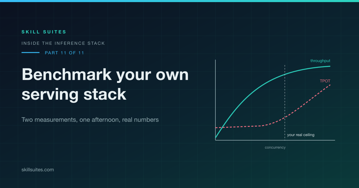
Throughput climbs steeply, then flattens. The flattening point is your real operating ceiling. Every request you admit past it buys queueing delay and nothing else. Note that the peak throughput number and the peak throughput concurrency are two different findings, and the second one is the more useful one.
TPOT stays nearly constant through the early levels. This is the important one. Going from 1 concurrent user to 8 should cost you almost nothing per token, because during decode the GPU spends its time reading weights out of memory and those weights get read once for the whole batch. That flat stretch is Part 9 made visible on your own hardware, and it is the result that surprises people who have never measured it.
TTFT rises, and the p99 rises faster than the p50. That divergence is the signal. Prefill compute affects both percentiles roughly equally. Queueing affects the tail first.
Definition
Saturation and the knee of the latency-throughput curve
Saturation is the concurrency at which added requests stop adding throughput. The knee sits a little before it: the last level at which latency is still nearly flat. The sweep reports the knee as the first level where p50 TPOT exceeds 1.5 times its batch-1 value.
Origin: the shape comes from queueing theory rather than from anything specific to LLMs. Mean waiting time in a simple single-server queue grows in proportion to 1 / (1 minus utilisation), so it stays nearly flat to roughly 70 percent utilisation and then turns vertical. Erlang derived results of this class for telephone exchange congestion in the 1910s, which is where the whole field starts.
Why it matters: the knee and peak throughput are different concurrency levels, often by a factor of two or more. Operating at peak throughput spends all your latency headroom to buy the last few percent of tokens per second.
Definition
Goodput
Throughput counted only over the requests that met their latency target. If a level serves 3,000 tok/s but a third of its requests blew a 500 ms TTFT budget, goodput at that SLO is 2,000 tok/s and the remaining 1,000 is work you cannot sell.
Origin: the word is borrowed from networking, where goodput has long meant the application-level payload rate once protocol overhead and retransmissions are excluded. LLM serving adopted it because peak throughput is reached at a concurrency where a large share of requests miss any tight latency target, so the raw figure overstates usable capacity.
Why it matters: a capacity plan built on peak throughput oversubscribes the box. Goodput at your real SLO is the number that survives contact with users.
The sweep does not compute goodput for you, and it does not need to. Pick your SLO, then walk the rows: any level whose p99 TTFT and p99 TPOT both sit inside the budget has goodput equal to its throughput, and the first level that fails the budget is where usable capacity stopped, whatever the throughput column says.
Which wall did you hit
When TPOT starts climbing you have hit one of two walls, and they need completely different fixes. The client numbers cannot separate them, because both walls bend the same curve the same way. The server log separates them in about thirty seconds.
- Look at the vLLM log for the level where TPOT broke. Not the client output. The server log.
- If you see preemption warnings (messages about a sequence group being preempted, or about cache blocks being swapped or recomputed), you ran out of KV cache. This is a memory problem, and it is the exact failure mode continuous batching and PagedAttention in Part 10 are designed to postpone. The scheduler admitted more sequences than it had blocks for, and it is now evicting and recomputing. The fixes are memory fixes: lower
--max-model-len, raise--gpu-memory-utilization, enable KV cache quantisation, or serve a smaller or more aggressively grouped model. - If the log is clean and GPU utilisation sits near 100 percent, you reached the compute knee. There is nothing to fix. You are using the card fully and the ridge point from script 01 should roughly agree with where this happened. If it does not agree, that disagreement is itself a finding worth chasing.
- Separately, check p99 TTFT against p50 TTFT. If p99 is pulling away from p50 while TPOT is still flat, that is queueing, not compute. Requests are waiting to be admitted. The fix is an admission control or concurrency cap in front of the server. A bigger GPU will not help.
Analogy
A p99 TTFT pulling away from p50 while TPOT stays flat is a supermarket where every till still scans items at exactly the same speed and the queues have simply grown. A faster scanner changes nothing. Another till, or letting fewer people through the door at once, changes everything.
Where it breaks: a shopper who reaches a till keeps it until they are done. The scheduler can preempt a sequence mid-decode and recompute it later, so a request can lose ground after it has already started being served, which no checkout does to anybody.
A client says the endpoint is slow. Anyone can run a load test. Telling them which of the three it is, KV cache or compute or queueing, from the log, in under a minute, is what the engagement is actually paying for.
Section takeaways
- Throughput climbs then flattens, and every request admitted past the flattening point buys queueing delay and no extra tokens per second.
- Flat TPOT from concurrency 1 to 8 is the memory-bound free lunch, because the weights are read from HBM once for the whole batch.
- Rising TPOT means one of two walls, and only the server log separates them: preemption or swap warnings mean KV cache, a clean log at near 100 percent utilisation means compute.
- p99 TTFT diverging from p50 while TPOT is flat is queueing, and the fix is admission control rather than a bigger card.
- The knee, reported as the first level where p50 TPOT exceeds 1.5 times its batch-1 value, sits below peak throughput and is the level you operate at.
Methodology hygiene, and what voids a run
Treat these as rules. Break any of them and your LLM serving benchmark produces a number that looks authoritative and means nothing.
- Randomise the prompts. If every request shares a prefix, prefix caching will serve most of the prefill from cache and your TTFT will look wonderful. Test that case deliberately if your workload has shared prefixes. Do not let it happen by accident.
- Force fixed output lengths. Without
min_tokensandignore_eos, some requests stop early and the levels are no longer comparable, because a level that happened to generate fewer tokens looks faster. - Warm up before measuring. The first requests at any concurrency level pay for CUDA graph capture, allocator growth and scheduler ramp. Discard them.
- Measure one card before you measure two. Two cards that disagree by more than a few percent on the same probe means a power or thermal issue, and every multi-GPU number you take after that inherits the problem.
- Report the context alongside every number. Model, quantisation, dtype, context length, prompt and output token counts, vLLM version, driver version, and every server flag. A throughput figure without that list is not a measurement. It is a rumour.
In practice
Four things void a run outright: prompts sharing a prefix when your traffic does not, output lengths allowed to vary, no warmup at a level, and any error count above zero that you did not open and read. A fifth voids it three months later, when nobody can reproduce it because the model, quantisation, context length, vLLM version, driver version and server flags were never written down. Write that config line into the same JSON file as the numbers, which is exactly what vars(args) is doing in the sweep script.
Honest caveats
These scripts are a starting point. They are not a finished harness, and you should expect to fix something small on the first run.
The most likely thing to break: if your vLLM version rejects min_tokens or ignore_eos, it predates them. Drop both fields from the payload. Output lengths will then vary a little more between requests, which is survivable as long as you say so when you report the numbers.
Also: results are specific to your model, your card, your driver version, your vLLM version and your flags. Change any one of those and rerun. A benchmark is a snapshot of a configuration, and treating it as a property of the hardware is how people end up quoting numbers that stopped being true two releases ago.
Section takeaways
- Shared prefixes plus prefix caching serve the prefill from cache, so TTFT improves for a reason your production traffic will not reproduce.
- Without
min_tokensandignore_eossome requests stop early, and a level that generated fewer tokens looks faster than it is. - The first requests at each level pay CUDA graph capture, allocator growth and scheduler ramp, which is why the client throws away up to 4 of them per level.
- Two identical cards disagreeing by more than a few percent on the same probe is a power or thermal fault, and every multi-GPU number taken afterwards inherits it.
- A result reported without model, quantisation, dtype, context length, versions and every server flag is a rumour, and it stops being true after two releases anyway.
Variations worth running
Each one is a single flag change, and each answers a question you would otherwise have to guess at.
| Question | The one change | What you learn |
|---|---|---|
| How much does context length cost me? | --prompt-tokens 128 vs 2048 vs 8192 |
How fast the KV cache eats your concurrency headroom |
| Does my workload have shared prefixes? | Server with and without --enable-prefix-caching |
Whether prefix caching is real money for you or a rounding error |
| Where does cache headroom cap me? | --gpu-memory-utilization 0.70 vs 0.95 |
The direct cache-size to concurrency curve |
| Does quantisation buy throughput? | Serve an AWQ or FP8 build of the same model | Throughput gain measured against quality loss |
| Tensor parallel or two replicas? | --tensor-parallel-size 2 vs two independent servers behind a load balancer |
The interconnect tax, on your box |
Run the last one early. Without NVLink, tensor parallelism pays an interconnect tax on every single layer, because each layer needs an all-reduce across the cards and that traffic crosses PCIe. Two independent replicas behind a load balancer share nothing and pay nothing, so they will usually win on throughput. They lose on maximum model size and on single-request latency, which is the real trade. “Probably” becomes “measured” in about twenty minutes, and if you are working through an on-prem hardware decision, this is the measurement that changes the purchase order.
Section takeaways
- Five variations, one flag each: prompt length, prefix caching,
gpu-memory-utilization, a quantised build, and tensor parallel against two replicas. - Sweeping prompt length across 128, 2048 and 8192 tokens measures how fast the KV cache eats the concurrency headroom that decides users per card.
- Without NVLink, tensor parallelism pays an all-reduce across PCIe on every one of the 80 layers, once per token.
- Two replicas behind a load balancer share nothing and usually win on aggregate throughput, and lose on maximum model size and single-request latency.
- Twenty minutes of measurement replaces the guess, and on an on-prem purchase it is the measurement that changes the order.
What to publish, and the number that gets forwarded
The artifact is small. Two plots, your measured ridge point, and four sentences explaining the shape of the throughput curve.
The last row is the one that gets forwarded. Take your peak sustained output throughput, multiply out to a million tokens, and divide by what the box costs to run for that long including power. Now you have a cost per million tokens for your hardware and your model, which you can put next to a hosted API price list. That number is what turns an LLM serving benchmark into a business argument, and it is the number missing from almost every writeup on the internet.
In practice
The number that goes in the capacity plan is throughput at the knee. Peak throughput is a separate finding and it belongs in the writeup rather than in the plan. Take the highest concurrency at which p50 TPOT is still inside 1.5 times its batch-1 value, read tokens per second at that level, divide by your median output length to get sustainable requests per second, and size the fleet on that. Then set the server’s concurrency cap at the same level, so the box is never allowed to run past the point you planned for.
Section takeaways
- The publishable artifact is two plots, the measured ridge point and four sentences on the shape of the throughput curve.
- Cost per million tokens is sustained tokens per second scaled up to a million, divided into what the box costs to run for that long including power.
- That single row is what makes an on-prem result comparable with a hosted API price list, which is the comparison people actually want.
- The ridge point from script 01 and the knee from script 02 should roughly agree, and a disagreement between them is a finding worth writing down rather than smoothing over.
Closing the series: ten parts, one plot
Every earlier part of this series contributes something to reading your own benchmark output.
- Part 1, the complete inference path: what a single request actually consists of, so you know what you are timing.
- Part 2, byte-pair encoding: tokens are the unit your benchmark counts, and tokens per second means nothing without knowing whose tokenizer.
- Part 3, inside one transformer block: the seven matrices, one of which is the exact
(B, 8192) @ (8192, 8192)shape script 01 measures. - Part 4, multi-head attention: where the KV cache comes from, which is what runs out first.
- Part 5, the output projection: another square projection with the same shape and the same memory behaviour.
- Part 6, the feed-forward network: where most of the weight bytes live, so most of what your decode step is reading.
- Part 7, mixture of experts: why an MoE model lands somewhere completely different on the same roofline plot.
- Part 8, the 2017 paper dissected: the reference figure, so you can map any architecture variant back to the shapes you are measuring.
- Part 9, the roofline model: the theory that script 01 turns into a number on your own card.
- Part 10, continuous batching and PagedAttention: the scheduler that produces the flat TPOT region, and the preemption warnings that explain where it ends.
Ten parts of theory. One afternoon of measurement. That is the honest way to benchmark LLM inference: the theory tells you what shape to expect, and the measurement tells you where your box actually stops, which is the only number you can build a plan on. If you are moving something from prototype to real traffic, that number belongs in the production readiness checklist before anything else.
Run it tonight. One LLM serving benchmark on your own hardware will teach you more by midnight than six months of reading other people’s charts.
Section takeaways
- Script 01 measures exactly the
(B, 8192) @ (8192, 8192)projection that Part 3 counted among the seven matrices of a block. - The flat TPOT stretch is Part 10’s continuous batching made visible, and the level where it ends is the level where the KV cache ran out of blocks.
- Tokens per second is only meaningful with a tokenizer attached, which is the Part 2 result showing up in a benchmarking table.
- Theory fixes the shape of the curve and measurement fixes the level, and only the level can be put in a capacity plan.
Key takeaways
- Take two measurements. The hardware roofline and the serving sweep. The gap between them is the finding.
- Sweeping batch size sweeps arithmetic intensity, because the weight matrix dominates the bytes moved. That makes the decode-batching argument measurable rather than assertable.
- Expect 10 to 20 percent below datasheet on bandwidth and peak. That shortfall is your real number, and it is what you should quote.
- TTFT, TPOT, end-to-end latency and throughput are four different things. Report p50 and p99 for the latency ones, never the mean.
- Flat TPOT means memory-bound and extra users are nearly free. Rising TPOT means you hit a wall, and only the server log tells you which one.
- p99 TTFT pulling away from p50 is queueing. Fix it with admission control. A bigger card will not help.
- Any LLM serving benchmark reported without model, quantisation, context length and server flags is not a measurement.
Frequently asked questions
What is the difference between TTFT and TPOT?
TTFT is the wall clock time from sending the request to receiving the first token, and it is dominated by prefill compute and by how long you waited in the queue. TPOT is the average gap between consecutive tokens after the first, and it is dominated by memory bandwidth and by how many sequences are decoding alongside you. They respond to different knobs, which is why a single latency number is useless.
Why is my measured memory bandwidth lower than the datasheet says?
A 10 to 20 percent shortfall is normal and expected. Datasheet bandwidth is a theoretical peak that assumes no refresh overhead, no ECC, and a perfectly streaming access pattern. Your measured figure is the one your model will actually get, so it is the one worth quoting.
How do I tell whether rising latency is a KV cache problem or a compute problem?
Read the server log at the concurrency level where TPOT started climbing. Preemption or swap warnings mean you exhausted the KV cache, which is a memory problem fixed with shorter context, more cache headroom or KV quantisation. A clean log with GPU utilisation near 100 percent means you reached the compute knee, which is not a problem at all.
Should I use tensor parallelism or run two independent replicas?
Measure it, because the answer depends on your interconnect. Without NVLink, tensor parallelism pays an all-reduce cost across PCIe on every layer, so two independent replicas behind a load balancer usually win on total throughput. Tensor parallelism still wins when the model does not fit on one card, or when single-request latency matters more than aggregate throughput.
Does prefix caching make my benchmark results look better than they are?
Yes, if your test prompts share a prefix and your real traffic does not. Randomise the prompts so prefill work is genuinely repeated, then run a second sweep with a deliberately shared prefix if that reflects your production workload. Reporting both is more honest than reporting either alone.
What concurrency limit should I actually set in production?
Set it at the point where TPOT stops being flat, which is usually well below the point of peak throughput. Past the flat region every additional admitted request buys queueing delay that your users feel and buys very little extra throughput in return.
Sources and further reading
- Roofline: An Insightful Visual Performance Model for Multicore Architectures, Williams, Waterman and Patterson, the original model that script 01 measures.
- Efficient Memory Management for Large Language Model Serving with PagedAttention, the vLLM paper, including the preemption and swapping behaviour you will see in the logs.
- vLLM documentation, for the current set of server flags, sampling parameters and the OpenAI-compatible API surface.
- GQA: Training Generalized Multi-Query Transformer Models from Multi-Head Checkpoints, on why KV cache size is the constraint that usually binds first.
- FlashAttention: Fast and Memory-Efficient Exact Attention with IO-Awareness, on why prefill behaves so differently from decode.
- torch.cuda.Event, the timing primitive used in the roofline probe.
Check your understanding
Take the 15 question quiz on this article
The same 15 questions every time, picked to cover every idea this article teaches, out of 30 written for it. The order of the questions and the order of the answer choices reshuffle on every attempt, so a retake never looks identical to the last one. It runs here on the page and keeps your place, so you can go and read a section and come back without losing anything. You get a full report at the end: your score, the correct answer to anything you missed, why it is correct, and a link straight back to the section it came from.
- 15 questions
- same set every time
- 8 knowledge areas
- hint on every question
- timed, no limit
