
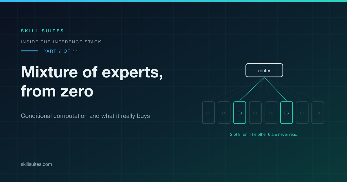
In a dense transformer, “knows more” and “costs more per token” are the same dial. Every parameter you add is another parameter that has to be dragged out of memory for every single token you generate. Mixture of experts breaks that link. It lets you add knowledge without adding per-token work, and that one sentence is the whole motivation.
Part 6 showed that the feed-forward network is where a transformer keeps most of what it knows. This part takes that slot and makes it conditional. By the end you should be able to look at “671B total, 37B active” on a model card and say exactly what it costs you in VRAM, in bandwidth and in cluster topology, why attention heads cannot be sparsified the same way, and why the advertised speedup is always roughly 4x and never exactly.
The running model is the one used everywhere else in this series: 80 layers, d_model 8,192, 64 query heads, 8 KV heads, FFN width 28,672. Every number below is small enough to check by hand.
- Part 1. How an LLM Answers a Question: The Complete Inference Path
- Part 2. Byte-Pair Encoding Explained: How LLMs Turn Text Into Tokens
- Part 3. Inside One Transformer Block: The Residual Stream and Its Seven Matrices
- Part 4. Multi-Head Attention Explained: Why 64 Heads Instead of One
- Part 5. The Output Projection: How 64 Attention Heads Become One Thought
- Part 6. The Feed-Forward Network: Where a Transformer Keeps What It Knows
- Part 7. Mixture of Experts Explained: Conditional Computation From Zero (you are here)
- Part 8. Attention Is All You Need, Dissected: The 2017 Figure, Box by Box
- Part 9. The Roofline Model: Why LLM Decode Is Memory-Bound
- Part 10. Continuous Batching and PagedAttention: How vLLM Keeps a GPU Busy
- Part 11. Benchmark Your Own LLM Serving Stack: Two Measurements, One Afternoon
Two dials instead of one
Bigger models know more. The trouble is that a dense model has one knob, and turning it up costs you on both axes at once: a 70B model holds more than a 7B model and reads ten times as many bytes per token to do it.

Mixture of experts gives you two knobs. Capacity grows with the number of experts. Per-token cost grows only with how many of them you choose to run.
Definition
Mixture of experts (MoE)
A layer holding many parallel sub-networks plus a small router that selects a few of them per token. With 8 experts and top-2 routing, six are skipped outright: their weights are never fetched and their arithmetic never runs. Attenuating them to a low weight instead would still cost the full read.
Origin: mixtures of local experts were described in 1991, where several small networks each specialised on part of the input space and a gating network combined them. The idea was brought into large neural language models in 2017 as a sparsely gated layer, specifically to grow capacity without growing the compute spent on each example.
Why it matters: it is the only place in a transformer where you can add parameters without adding per-token bytes, and it is why a model card now needs two parameter counts where a dense one needed a single number.
Structurally, experts and attention heads are the same idea. Partition a representation into parts, let each part specialise, recombine the results. Heads do it with 64 slices and W_O. Experts do it with N sub-networks and a weighted sum. One switch separates them, and it is whether a selection step exists at all.
Dense means no selection step exists
All 64 heads run on every token, at every layer, always. Nothing decides which ones. There is no mechanism by which head 37 could sit out this token, so every byte of every attention weight is read for every token, unconditionally.
Sparse means a router picks
Replace the single feed-forward network with eight, put a small scoring matrix in front, and keep the top two. Now the input decides which parameters run. Six of the eight are never fetched from HBM, so their bytes never move and their arithmetic never happens.
Definition
Conditional computation
Any arrangement where the input decides which parameters run. Top-2-of-8 routing qualifies, because six sets of weights are never touched. Multiplying an expert’s output by a weight of 0.01 does not qualify, because the weights were still read to produce it.
Origin: the term comes from deep learning research in the early 2010s on letting a network’s capacity grow while the cost per example stayed flat. The 2017 sparsely gated mixture-of-experts layer was the first version of it that held up at language-model scale.
Why it matters: it is the single test that separates sparse from dense, and it is why 64 attention heads count as dense even though they look like 64 specialists.
Section takeaways
- Dense scaling moves capacity and per-token bytes together, so a 70B model reads about ten times the bytes per token that a 7B model reads.
- MoE splits that into two dials: capacity grows with the expert count, per-token cost grows only with how many experts run.
- Heads and experts share the same partition, specialise, recombine shape, and differ only in whether a selection step exists.
- All 64 attention heads run unconditionally at every layer, so no head can sit out a token.
- With 8 experts and top-2 routing, six experts are never fetched from HBM, and that skipped read is the entire source of the saving.
The slot it replaces, and what an expert is
Mixture of experts almost never touches attention. It replaces step 9 of the block from Part 6, the feed-forward network, and leaves the residual stream, the norms, the projections and the KV cache exactly as they were. Running the parameter count for the running example, a Llama-3-70B class model with d_model 8,192, 64 query heads, 8 KV heads and FFN width 28,672, shows why that slot and no other:
attention   W_Q  8192 x 8192  =  67.1M
            W_K  8192 x 1024  =   8.4M
            W_V  8192 x 1024  =   8.4M
            W_O  8192 x 8192  =  67.1M
attention subtotal             = 151.0M

FFN     3 matrices, 8192 x 28672 each
                               = 704.6M

layer total                      855.6M
FFN share  704.6 / 855.6       =  82.4%
The FFN holds roughly 82 percent of a layer’s parameters, and it is also the only large component that processes each token independently, with no mixing across positions. That combination makes it both the biggest prize and the easiest thing to split: a routing decision for one token has no consequences for any other token in the sequence.
An expert is a copy of the FFN
Definition
Expert
One complete copy of the feed-forward network: a gate matrix, an up matrix, a down matrix, and a nonlinearity between them. Eight experts in the running example means eight sets of those three matrices, differing only in their learned values.
Origin: the name is inherited from the 1991 mixture-of-local-experts work, where each sub-network was expected to become good at one region of the input space. Inside a transformer an expert is the FFN sublayer duplicated rather than a separate model.
Why it matters: no new machinery is involved, so the whole cost and the whole benefit of MoE come from how many copies exist and how many of them the router runs.
A dense layer has one expert. An MoE layer has eight, or sixty-four, or two hundred and fifty-six.
Analogy
A firm with eight specialists on retainer. Each case goes to two of them and the other six bill nothing that day, while the firm still pays to keep all eight on the books.
Where it breaks: a client receives one specialist’s answer and can tell whose it was. Here the two outputs are blended at 0.668 and 0.332 into a single 8,192-wide vector, and nothing downstream can recover which expert contributed what.
Section takeaways
- MoE replaces the feed-forward slot alone and leaves attention, the norms, the residual stream and the KV cache untouched.
- The FFN is 704.6M of a layer’s 855.6M parameters, which is 82.4 percent, against 151.0M for all four attention matrices.
- The FFN is the only large component that handles each token independently, so routing one token has no consequence for any other token in the sequence.
- An expert is the same three matrices Part 6 described, so eight experts multiply the slot’s parameters by eight and change no shape anywhere else.
The router, with real numbers
Definition
Router (gating network)
The small matrix in front of the experts, d_model by n_experts, that scores every expert for the current token. At 8,192 x 8 it is 65,536 parameters standing in front of roughly 5.6 billion parameters worth of experts.
Origin: a gating network was part of the original 1991 mixture-of-experts formulation, where it produced a weight for every expert and all of them ran. The 2017 sparsely gated layer made the gate keep only the top few weights, which is what turned a blending scheme into a way of skipping work.
Why it matters: it is about 0.001 percent of the layer and it decides everything. A router that collapses onto one expert leaves you paying to store the other seven for nothing.
The router multiplies the token’s vector and produces one score per expert. Those are the router logits. Take the top two, then softmax over those two and only those two:
logits    E1 1.2   E2 3.8   E3 0.4   E4 2.1
          E5 4.5   E6 0.9   E7 1.6   E8 2.3

top-2     E5 (4.5) and E2 (3.8)

e^4.5  =  90.0
e^3.8  =  44.7
sum    = 134.7

gate(E5) = 90.0 / 134.7 = 0.668
gate(E2) = 44.7 / 134.7 = 0.332
Definition
Top-k routing
Keeping the k highest router logits, running only those k experts, and softmaxing over the k selected scores alone. Mixtral uses k of 2 out of 8 experts. DeepSeek-V3 uses k of 8 out of 256 routed experts.
Origin: introduced with the 2017 sparsely gated layer, which kept the top k of n gate values so that most experts could be skipped entirely. Switch Transformers pushed k down to 1 in 2021 to cut routing cost and simplify the implementation.
Why it matters: k is the dial that sets active parameters. Raising it by one adds a whole expert’s bytes to every token, at every layer, for the life of the deployment.
That the softmax runs over the selected pair and not over all eight changes the arithmetic. Normalised over all eight logits, E5 would come out around 0.55 and E2 around 0.27, and the two would sum to about 0.82 rather than 1.00. The scale of the layer’s output would then wobble from token to token depending on how confident the router happened to be. Normalising over the chosen pair pins the sum at 1.00 every time, so the blended output has the same scale a dense FFN would have produced. The residual stream never notices that anything changed.
One token through the layer, state by state
Watch what happens to experts 1, 3, 4, 6, 7 and 8 in the complete pass below, which is nothing at all.
| State | Size | What happened |
|---|---|---|
x |
8,192 | arrives from the norm, same as always |
| logits | 8 | one score per expert, from W_router |
| selected | 2 of 8 | E5 and E2 |
| gates | 2 | 0.668 and 0.332, summing to 1.00 |
| out | 8,192 | 0.668 x E5(x) + 0.332 x E2(x) |
| E1, E3, E4, E6, E7, E8 | none | weights never fetched from HBM |
Section takeaways
- The router is one 8,192 x 8 matrix, 65,536 parameters in front of roughly 5.6 billion parameters of experts.
- Top-2 of the eight logits survive, and with scores 4.5 and 3.8 the gates come out at 0.668 and 0.332, summing to exactly 1.00.
- Normalising over all eight instead would have given about 0.55 and 0.27, a sum near 0.82, and an output scale that moved with router confidence.
- The layer emits a single 8,192-wide vector, so nothing downstream of the FFN slot can tell that the layer was sparse.
- Six of the eight experts have their weights left in HBM, which is what the router bought.
Total versus active parameters
Definition
Total versus active parameters
Total is everything that has to be resident in memory. Active is what gets read to produce one token. DeepSeek-V3 is 671B total and 37B active. A dense model quotes one number because for it the two are equal.
Origin: the pair became standard vocabulary when sparse models began shipping with two counts on the model card, as in the 2024 Mixtral report quoting about 47B total against about 13B active.
Why it matters: total sizes your GPUs and active sizes your latency. Confusing them is the most common error people make about mixture of experts, and it is the one that ends with a model that will not load.
| Model | Total parameters | Active per token | Routing |
|---|---|---|---|
| Llama-3-70B (dense) | 70B | 70B | none, active equals total |
| Mixtral 8x7B | about 47B | about 13B | 8 experts, top-2 |
| DeepSeek-V3 | 671B | 37B | 256 routed experts top-8, plus 1 shared |
Mixture of experts does not reduce how much memory you need. All 671B of DeepSeek-V3 must be loaded, which is roughly 1.3 TB at fp16 before you allocate a single byte of KV cache. What falls is how much you read per token. You get the capacity cost of a 671B model and the per-token speed of a 37B one.
Quantization is the obvious lever on that first number, and it works on an MoE exactly as on dense weights. The same 671B at 4 bits is roughly 336 GB rather than 1,342 GB, the difference between a rack and a node. It moves the VRAM bill without touching the argument, because the per-token read falls by the same factor:
            resident (total)      read per token (active)
fp16          1,342 GB                    74 GB
4-bit           336 GB                    18 GB
Sparsity and quantization are orthogonal. One decides which weights you touch, the other decides what each weight costs, and serving a frontier MoE in practice means doing both.
In practice
Size the GPUs off the total parameter count and size the latency off the active one. A 671B model at fp16 needs roughly 1.3 TB of memory whether 37B or 671B of it gets read per token, and the KV cache comes on top of that. A capacity plan that quotes the active number for VRAM produces a cluster the weights do not fit on.
Why fewer bytes means less time
At small batch, decode is memory-bound. The arithmetic units sit mostly idle while weights stream in from HBM, and step time is set by bytes moved and almost nothing else. That makes skipping weights a bandwidth optimisation wearing an architecture costume, and it is the load-bearing connection to Part 9 and the roofline model.
Take the Mixtral-shaped numbers. A dense 47B model at bf16 is 94 GB of weights, all of which must cross the memory bus for every token. The MoE version reads about 13B, or 26 GB. An H100 SXM part delivers about 3.35 TB/s, so take a round and slightly conservative 3 TB/s: that is about 31 ms per token against about 9 ms. Same knowledge in the model, 3.6x fewer bytes on the wire, roughly 3.6x less time.
If decode were compute-bound, the bytes you skipped would not be on the critical path at all. You would still save the arithmetic of six experts, and that is worth something. The dramatic part, the part that turns 94 GB into 26 GB and a 31 ms step into a 9 ms one, exists only because memory was the constraint.
Section takeaways
- Total parameters set the VRAM bill and active parameters set the per-token read, and MoE lowers only the second.
- DeepSeek-V3 is 671B total and 37B active, roughly 1.3 TB at fp16 before any KV cache is allocated.
- Mixtral 8x7B is about 47B total and about 13B active, from 8 experts with top-2 routing.
- At batch 1 the dense 47B reads 94 GB per token and the sparse version reads 26 GB, about 31 ms against about 9 ms at 3 TB/s.
- The win is a bandwidth win: in a compute-bound regime the skipped bytes are off the critical path and the same trick buys far less.
Routing collapses unless you stop it
There is a feedback loop hiding in this design. An expert that starts marginally better gets picked marginally more, therefore receives more gradient, therefore improves faster, therefore gets picked more still. Rich gets richer.
Left alone, one expert absorbs nearly all traffic within a few thousand training steps and the other seven never learn anything.
Definition
Load-balancing auxiliary loss
An extra penalty term added to the training objective, proportional to how uneven expert usage is across a batch. It says nothing about output quality. Its only job is keeping all eight experts in use.
Origin: auxiliary balancing losses arrived with the 2017 sparsely gated layer, which had to break the self-reinforcing loop in which a few experts won all the traffic. Switch Transformers reduced it to a single differentiable load-balancing term in 2021.
Why it matters: without it, one expert absorbs nearly all routing within a few thousand steps, and you have paid the storage bill for seven experts that never learned anything.
Alongside the auxiliary loss sits expert capacity, a per-expert cap on how many tokens it will accept in a batch. It exists because each expert’s input buffer is a fixed-size allocation, so a batch that sends one expert more tokens than the cap has nowhere to put them. Tokens beyond the cap are dropped, which means they skip the FFN entirely and pass through on the residual alone. A dropped token is not an error the model reports. It is a token that quietly received less computation than its neighbours.
Scope that to training before you hunt for it in production. Inference stacks run these models dropless, with the capacity factor switched off, so every token reaches its experts. Imbalance still costs you, but as a slower step while one device drains a longer queue, not as a token that silently got less compute.
Newer models have moved away from the auxiliary loss because it fights the language-modelling objective for gradient. DeepSeek-V3 uses an auxiliary-loss-free scheme instead: a per-expert bias term added to the routing scores before top-k selection, nudged up or down during training to even out load without contributing any gradient of its own.
Expert-choice versus token-choice routing
Everything above describes token-choice routing, where each token picks its experts and balance is only a hope. Expert-choice routing inverts the selection: each expert picks its top-k tokens from the batch, so balance holds by construction and no auxiliary loss is needed. It pays for that with uneven token coverage and a need for the whole batch in view, which is awkward for autoregressive decoding.
Section takeaways
- Routing carries a rich-gets-richer loop: more traffic gives an expert more gradient, which earns it more traffic.
- Left unchecked, one expert takes nearly all routing within a few thousand steps, and by step 5,000 the partition is dead.
- The load-balancing auxiliary loss penalises uneven usage across a batch and contributes nothing to output quality.
- Expert capacity caps tokens per expert per batch because the input buffer is a fixed allocation, and tokens over the cap skip the FFN and travel on the residual alone.
- DeepSeek-V3 replaces the auxiliary loss with a per-expert bias added before top-k selection, so balancing costs no gradient.
- Expert-choice routing balances by construction and pays for it with uneven token coverage and a need for the whole batch in view.
Shared experts, fine-grained experts, and where they live
Fine-grained experts means many small experts rather than a few large ones. DeepSeek-V3 runs 256 routed experts and picks 8. Choosing 8 of 256 admits about 4 x 10^14 distinct expert combinations, against the 28 that 2-of-8 allows, and each combination is a different function the layer can apply to a token.
Shared experts run on every token with no routing decision at all, absorbing the general-purpose work so the routed experts stop spending their capacity relearning the same common cases.
Definition
Shared expert
An expert that every token runs, with no routing decision involved, sitting alongside the routed ones. DeepSeek-V3 runs 1 shared expert next to the 8 routed experts it selects from 256.
Origin: set out in DeepSeek’s 2024 mixture-of-experts work as shared expert isolation, adopted because every routed expert was otherwise spending part of its capacity relearning the same common cases.
Why it matters: a shared expert is unconditional, so its bytes land in the active parameter count for every single token, and it is one of the reasons a measured speedup falls short of the routing ratio.
Where experts physically live
671B parameters do not fit on one GPU, or on eight. Mixture of experts at that scale is served with expert parallelism: experts are distributed across devices, and tokens are shipped over the network to whichever GPU holds their chosen expert, then shipped back. That is an all-to-all exchange, and it happens twice per MoE layer, once to dispatch and once to combine.
Definition
Expert parallelism
Splitting a layer’s experts across devices so each GPU holds a subset, then shipping every token to whichever GPU holds its chosen expert and shipping the result back. That is two all-to-all collectives per MoE layer, one to dispatch and one to combine.
Origin: the pattern comes from 2020 work on scaling mixture-of-experts transformers across accelerators, where the experts of one layer were sharded over devices and an all-to-all collective moved tokens to them. It exists because a frontier MoE layer does not fit on any single device.
Why it matters: it turns interconnect bandwidth into a serving parameter, and it turns expert load imbalance into GPU load imbalance, where one device’s queue stalls every other device waiting on the collective.
Two all-to-all exchanges per MoE layer means 80 MoE layers would put 160 collectives on the critical path of every single decode step, and each collective runs at the speed of its slowest participant. Treat 160 as the upper bound, because it assumes every layer is an MoE layer and real models do not do that. DeepSeek-V3 has 61 layers and keeps the first 3 dense, which is 58 MoE layers and 116 collectives per step.
In practice
If you are weighing a move to self-hosted inference, expert parallelism is the line item that separates “we can serve a 70B dense model on one node” from “we need a fabric”. On two GPUs, with a model that already fits, a dense model is usually the better engineering choice.
Section takeaways
- Fine-grained routing means many small experts, and DeepSeek-V3’s 8-of-256 admits about 4 x 10^14 combinations against the 28 that 2-of-8 allows.
- A shared expert runs on every token with no routing decision, so routed experts stop relearning the common cases.
- Because a shared expert is unconditional, its bytes count as active parameters on every token.
- Expert parallelism shards experts across devices and pays two all-to-all collectives per MoE layer, so DeepSeek-V3’s 58 MoE layers carry 116 collectives per decode step.
- Expert load imbalance becomes GPU load imbalance, where one slow device stalls every other device on the collective.
Three honest caveats
1. Why heads cannot be sparsified the same way
If skipping is so good, the obvious follow-up is why not skip attention heads too. Both are partition, specialise, recombine. Only one of them gets the benefit, and the reason is memory layout rather than concepts.
W_Q in the running example is one 8,192 x 8,192 matrix, a single contiguous 134 MB allocation. Head 6 is not a separate tensor. It is columns 768 through 895 of that matrix’s output, sliced after the multiply. To skip head 6 you would still issue the same read of the same block, because the read is one operation over one address range. The bytes are already in flight before any head exists.
Analogy
Attention heads are columns on one printed page. Experts are separate leaflets in a rack. You can leave a leaflet in the rack, and you cannot leave a column on a page you have already picked up.
Where it breaks: with a page you could at least skip a column with your eyes and save the reading time. A GPU cannot, because the read is issued over an address range, so head 6’s bytes have crossed the bus before any code could decide head 6 was unwanted.
Experts are different in exactly the way that matters: each one is a separately allocated tensor with its own address. Not issuing the read genuinely avoids moving the bytes. This is the same mechanical sympathy argument you meet anywhere memory layout decides performance, applied to a transformer.
2. Why batching erodes the advantage
One token reads 2 of 8 experts. The GPU has to load every expert that any token in the batch selected, and the union grows fast. One token misses a given expert with probability 6/8, so across a batch of B tokens the expected number of distinct experts read is 8 * (1 - 0.75^B):
batch  1    2.0 of 8   read  ( 25% )
batch  4    5.5 of 8   read  ( 68% )
batch  8    7.2 of 8   read  ( 90% )
batch 16    7.9 of 8   read  ( 99% )
batch 64    8.0 of 8   read  (100% )
By batch 16 you are reading essentially the whole layer and the bandwidth saving is gone. The FLOP saving survives, because each token still only computes through two experts. The byte saving does not, because the weights get loaded regardless of who asked for them.
Two assumptions sit under that table and only one is safe. Even routing is engineered, which is what the load-balancing loss buys. Independent routing is not: a trained router sends similar tokens to the same experts, so real selections cluster and the true union grows more slowly than the formula says. Read the table as the fastest the advantage can collapse, not as a measurement of your workload.
Analogy
A museum with eight rooms where every visitor is booked into two of them. One visitor and six rooms stay dark. Sixteen visitors and somebody is in every room, so every light is on.
Where it breaks: the lighting bill covers the bytes and nothing else. Each visitor still walks through exactly two rooms however big the crowd gets, which is why the arithmetic saving survives batching while the bandwidth saving does not.
Fine-grained routing pushes the crossover further out. With 256 experts and top-8, a batch of 64 reads roughly 220 of 256, so there is still headroom, but the effect remains. The practical consequence is that MoE’s latency advantage is largest at low concurrency and shrinks under load, which interacts directly with how you think about batch size, queueing and tail latency. It is also why MoE serving pushes toward spreading experts over many GPUs rather than packing batches onto few.
3. Why the speedup is “roughly” 4x and never exactly
Skip 6 of 8 experts and the expert portion of the read drops by 4x. The step does not, because the expert portion is not the whole step. Attention weights are read in full. Embeddings are read in full. The router is small but not free. The KV cache is read every step and grows with sequence length. A shared expert, if the model has one, runs on every token by definition.
The parameter accounting makes this concrete without any hardware in the picture. Mixtral is quoted at 47B total and 13B active. 47 divided by 13 is 3.6, not 4, and the gap is exactly the attention and embedding parameters that were never skippable. Add the KV cache and the router on top and you land lower still.
Achieved bandwidth leaks more of it. A dense FFN is one large contiguous read, the shape memory systems are happiest with. An MoE layer gathers two smaller expert tensors from scattered addresses and runs a narrow multiply on each, so read and arithmetic both sit further from peak. 3.6x is the byte ratio. What you measure lands under it.
In practice
Read any “4x faster” attached to a top-2-of-8 model as an upper bound on one component of the step rather than a measured end-to-end number. What you actually get depends on your batch size, your sequence length, your interconnect and the quality of your MoE kernels, so measure it on your own stack, which is what Part 11 is for.
Section takeaways
W_Qis one contiguous 8,192 x 8,192 allocation of 134 MB, so head 6 is columns 768 to 895 of a read that was issued as a single operation.- Experts are separately allocated tensors, so declining to issue the read genuinely keeps their bytes off the bus.
- With 8 experts and top-2, the expected distinct experts read is
8 * (1 - 0.75^B): 2.0 at batch 1, 5.5 at batch 4, 7.9 at batch 16. - The FLOP saving survives batching because each token still computes through two experts. The byte saving does not.
- With 256 experts and top-8, a batch of 64 still reads only about 220 of 256, so fine-grained routing moves the crossover without removing it.
- Mixtral’s 47B over 13B is 3.6x, and the shortfall from 4x is the attention, embedding, router and KV-cache bytes that were never skippable.
What counts as dense, and the trade in full
The test is a single question. Does the input decide which parameters run? If no, the computation is dense: every parameter participates, active equals total, and no router exists. If yes, you are in conditional-computation territory regardless of how many parts end up running.
Attention heads are dense. Dense FFNs are dense. Embeddings and norms are dense. In a standard transformer, MoE experts are the only sparse component, which is why “sparse model” is a claim about one slot in the block and not about the model as a whole.
Dense FFN versus MoE FFN, side by side
Instantiate the whole trade on a 47B-class model at bf16, and the decision falls out of two rows:
| Property | Dense FFN | MoE FFN (8 experts, top-2) |
|---|---|---|
| Parameters in the slot | 1x | 8x |
| Model-level total | 47B | 47B, mostly experts |
| Active per token | 47B, all of it | about 13B |
| Bytes read per token | 94 GB | 26 GB at batch 1 |
| Router overhead | none | one d_model x 8 matrix, about 0.001% of the slot |
| KV cache impact | baseline | identical, because MoE replaces the FFN and never touches W_K or W_V |
| VRAM to hold the model | 94 GB | 94 GB, unchanged |
| Throughput at batch 1 | baseline | roughly 3.6x more tokens per second |
| Throughput at large batch | baseline | advantage erodes toward parity as the expert union fills |
| Serving topology | tensor parallel is enough | expert parallelism plus two all-to-all exchanges per layer |
| Training | standard | needs load balancing, routing can destabilise |
| Fine-tuning | well understood | harder, routing can shift under you |
The fine-tuning row is the one that catches teams late. Updating the experts also shifts what the router prefers, so a model that fine-tuned cleanly can come back with a different load distribution, and therefore a different latency profile, than the one you benchmarked.
Read the VRAM row and the throughput row together and you have the entire trade. You buy the speed of a small model and you pay the storage bill of a large one. Whether that is a good deal depends almost entirely on your concurrency, which is the thread Part 10 picks up when it looks at how a scheduler keeps a GPU busy.
Section takeaways
- One question decides sparse from dense: does the input choose which parameters run.
- Attention heads, dense FFNs, embeddings and norms all fail that test, so MoE experts are the only sparse component in a standard transformer.
- The MoE slot holds 8x the dense slot’s parameters and reads about 13B of 47B per token at batch 1.
- VRAM is 94 GB either way, while bytes read per token fall from 94 GB to 26 GB at batch 1 and climb back toward 94 GB as the batch grows.
- The router costs one
d_modelx 8 matrix, about 0.001 percent of the slot, and the KV cache is untouched because attention was never modified.
Key takeaways
- Mixture of experts separates how much a model knows from how much work each token costs, by letting the input choose which parameters get read.
- It replaces the FFN slot only. The FFN holds about 82 percent of a layer’s parameters and processes each token independently, which makes it the biggest prize and the easiest thing to split.
- An expert is a plain copy of the FFN. The router is one
d_modelbyn_expertsmatrix, and the softmax runs over the selected experts alone so the gate weights always sum to 1.00. - Total parameters set your VRAM bill. Active parameters set your per-token speed. MoE lowers the second and leaves the first exactly where it was.
- The win is a bandwidth win. It only looks this good because decode at small batch is memory-bound, and it shrinks as batch size grows and the union of selected experts fills up.
- Heads cannot be sparsified the same way because they are slices of one contiguous matrix. Experts are separate allocations, which is the only reason skipping them saves anything.
- At frontier scale MoE is an infrastructure decision. Expert parallelism and two all-to-all exchanges per layer make interconnect a first-class serving parameter.
Frequently asked questions
Does mixture of experts reduce the VRAM needed to serve a model?
No. Every parameter still has to be resident, so a 671B total model needs roughly 1.3 TB at fp16 whether or not it is sparse. What falls is bytes read per token, which is a bandwidth saving rather than a capacity saving.
How many experts are active per token in Mixtral and DeepSeek-V3?
Mixtral 8x7B routes each token to 2 of its 8 experts, giving roughly 13B active out of about 47B total. DeepSeek-V3 routes each token to 8 of 256 routed experts and also runs 1 shared expert on every token, giving 37B active out of 671B total.
Why does an MoE model lose its speed advantage at high batch size?
The GPU must load every expert that any token in the batch selected, so what matters is the union across the batch rather than the count per token. With 8 experts and top-2 routing, a batch of 16 already reads about 7.9 of 8, so the bandwidth saving is essentially gone.
Does MoE change the size of the KV cache?
No. The KV cache is produced by the key and value projections inside the attention block, and MoE replaces the feed-forward slot without touching attention. Cache size still depends on layers, KV heads, head dimension and sequence length exactly as it did before.
Can you run an MoE model on a single GPU?
Only if the total parameter count fits in that GPU’s memory, since active parameters have nothing to do with what must be resident. Models like DeepSeek-V3 require expert parallelism across many devices, with tokens routed over the interconnect to whichever GPU holds their chosen expert. The exception is expert offloading, where experts live in system RAM or on NVMe and only the selected ones cross PCIe per token, which is how Mixtral 8x7B runs on one consumer card at a large speed penalty.
Why is the speedup described as roughly 4x rather than exactly 4x?
Only the expert portion of the read is skippable. Attention weights, embeddings, the router and any shared expert are read on every token, and the KV cache is read every step, so the whole-step ratio always comes out below the expert-level ratio.
Sources and further reading
- Outrageously Large Neural Networks: The Sparsely-Gated Mixture-of-Experts Layer, the paper that introduced the gated expert layer.
- Switch Transformers, for top-1 routing, expert capacity and the load-balancing loss in its standard form.
- Mixtral of Experts, the 8x7B model behind the 47B total and 13B active numbers used throughout this part.
- DeepSeek-V3 Technical Report, for fine-grained experts, shared experts and the auxiliary-loss-free balancing strategy.
- Transformer Feed-Forward Layers Are Key-Value Memories, on why the FFN slot is where the knowledge lives.
- vLLM documentation, for how expert parallelism and MoE serving are configured in practice.
Next: Part 8 goes back to the 2017 figure and reads it box by box, now that every box in it has a name.
Check your understanding
Take the 15 question quiz on this article
The same 15 questions every time, picked to cover every idea this article teaches, out of 30 written for it. The order of the questions and the order of the answer choices reshuffle on every attempt, so a retake never looks identical to the last one. It runs here on the page and keeps your place, so you can go and read a section and come back without losing anything. You get a full report at the end: your score, the correct answer to anything you missed, why it is correct, and a link straight back to the section it came from.
- 15 questions
- same set every time
- 8 knowledge areas
- hint on every question
- timed, no limit
