
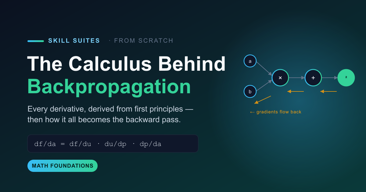
The calculus behind backpropagation is smaller than almost anyone admits. Not a semester of it. Maybe fifteen percent of a first calculus course, derived from a single idea, plus one rule that isn’t in single-variable calculus at all. Master that slice and backpropagation stops being a magic incantation you import and becomes something you can do on paper. This article builds that slice from the floor up — every derivative derived, not memorized — with worked examples, exercises you can try, and then the payoff: watching the exact same math turn into the backward pass.
It is the mathematical companion to How Neural Networks Learn, which walked the training loop end to end but deliberately hand-waved the calculus with a promise to come back to it. This is coming back to it.
A test you should be able to pass with a pen
Before the teaching, a diagnostic. Here is a tiny problem. Try it before you read on.
a = 2,  b = -3,  c = 1
f = (a*b + c)^2

Compute  df/da,  df/db,  df/dc  by hand.
The forward value is easy: a·b = −6, +c = −5, (−5)² = 25. The gradients are where it gets interesting. A very common attempt looks like this — take the derivative of the square, 2×(−5) = −10, then divide by the input you’re differentiating against:

| Attempt | Value | Correct | Verdict |
|---|---|---|---|
| df/da = 2(−5) ÷ 2 | −5 | 30 | wrong |
| df/db = 2(−5) ÷ (−3) | 3.33 | −20 | wrong |
| df/dc = 2(−5) ÷ 1 | −10 | −10 | right |
Two of three are wrong — the method divides where it should multiply. But look at the third row. It is correct. And it is correct by coincidence: the method divided by c, and c happened to be 1, so dividing by 1 and multiplying by 1 give the same number. The broken process returned the right answer.
A wrong process that returns a right answer is not a right process. It is a right process that has not failed yet. If you had only checked df/dc, you would have concluded you understood backpropagation and moved on — carrying a broken method into every harder problem, where c is not 1 and the coincidence does not save you. Memorized rules fail silently. Derived understanding does not.
So we are going to derive it. By the end, the correct answers — 30, −20, −10 — will be something you can produce and defend, and you will see that producing them is exactly what backpropagation does.
Concept 1 — A derivative is a nudge ratio
Forget every rule you have seen. A derivative answers one question: if I nudge the input by a tiny amount, how much does the output move? It is rise over run. To measure a slope you need two points: one at x, one a tiny step h to the right at x + h.
run   = (x + h) - x        = h
rise  = f(x + h) - f(x)
slope = rise / run         = [ f(x+h) - f(x) ] / h
Then shrink h toward zero, so the two points collapse into one and you get the slope at that exact spot rather than an average across a gap. That is the whole of differential calculus, in one line — the limit definition:
f′(x) = limh→0 [ f(x+h) − f(x) ] / h
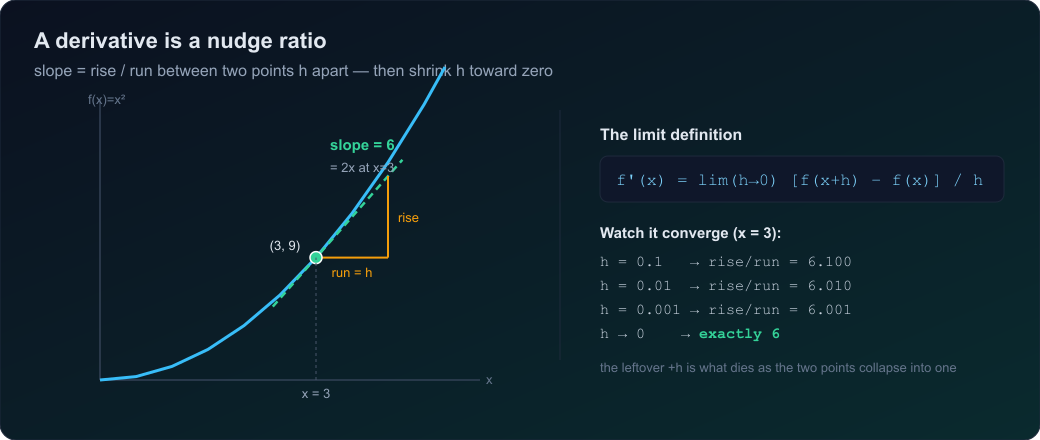
Notation: f′(x) and df/dx mean the same thing. The d means “an infinitely small change in,” so df/dx literally reads: tiny change in f, divided by tiny change in x. A ratio. Not a rule to memorize — the source of every rule below.
Concept 2 — The power rule is a count, not a rule
Take f(x) = x² and apply the definition literally. The only algebra you need is expanding (x + h)²:
f(x + h) = (x + h)^2 = x^2 + 2xh + h^2

rise   = (x^2 + 2xh + h^2) - x^2   =   2xh + h^2
/ run  = (2xh + h^2) / h           =   2x + h
h -> 0                             =   2x
Three things happened, and each has a reason worth naming:
- x² cancelled — of course it did. It is the starting height, and the starting height cannot be part of the rise.
- one h cancelled — because slope is rise over run, and the run is
h. - the leftover + h died — shrink
hto nothing and it is gone.
Now do x³. Same procedure, one more term in the expansion:
(x + h)^3 = x^3 + 3x^2 h + 3x h^2 + h^3

rise   =        3x^2 h + 3x h^2 + h^3
/ h    =        3x^2   + 3x h   + h^2
h -> 0 =        3x^2
The pattern is now visible: the derivative is the coefficient of the single-h term. Everything with h² or higher is tiny×tiny and dies; everything with no h is the starting height and cancels. Only the middle survives. And why is that coefficient 3 for x³? Because when you expand (x+h)³ there are three slots to pull the single h from, and the other two slots each contribute an x. That is the power rule:
xⁿ → n · xⁿ⁻¹
The n out front is a count of slots. The “minus one” in the exponent is the power of x that the ÷ h consumed. The power rule was never handed down from a mountain — it is a count you can re-derive any time you doubt it.
Concept 3 — Constants die
A constant is a flat horizontal line. Nudge x, nothing moves, rise is zero, slope is zero. From the definition in one line: f(x+h) − f(x) = 5 − 5 = 0, and 0 / h = 0. This is why x² and x² + 11 have the identical derivative: adding 11 lifts the whole curve 11 units without changing its steepness anywhere. Constants shift; they never tilt.
With the power rule, constants dying, and the fact that a sum differentiates term by term, you can already handle any polynomial. 6x⁵ − 2x² + 11 → 30x⁴ − 4x. Bring each exponent down, drop it by one, and let the lone constant vanish.
Do these with a pen before revealing the answers. Say each exponent out loud so it does not go missing.
f(x) = x⁷f(x) = 4x³f(x) = x² + 5x − 9f(x) = 6x⁵ − 2x² + 11- From the definition only (no rules): derive the derivative of
f(x) = x² + 3x.
Show worked answers
1.  x^7            -> 7x^6                      (bring down 7, exponent 7-1=6)
2.  4x^3           -> 12x^2                     (4 * 3x^2; the 4 is a passenger)
3.  x^2 + 5x - 9   -> 2x + 5                    (5x -> 5, the -9 dies)
4.  6x^5 - 2x^2+11 -> 30x^4 - 4x                (the +11 dies)
5.  f(x+h) = (x+h)^2 + 3(x+h) = x^2 + 2xh + h^2 + 3x + 3h
    minus f(x)     = 2xh + h^2 + 3h
    / h            = 2x + h + 3
    h -> 0         = 2x + 3
Check #5 by nudging at x = 4: f(4)=28, f(4.001)=28.011001, rise/run = 11.001 → 2(4)+3 = 11. The stray .001 is the +h that dies.
Concept 4 — The chain rule is multiplication, never division
This is the one the diagnostic caught, so let us be exact. The power rule handles x⁵. It does not handle (3x + 1)⁵, because the thing being raised to a power is not x — it is another whole function. A function inside a function is a composition, and it needs its own rule. If f depends on u, and u depends on a:
df/da = df/du · du/da
Why a product? Think of derivatives as exchange rates. du/da = 3 means one unit of a buys three units of u. df/du = 2 means one unit of u buys two units of f. So one unit of a buys 3 × 2 = 6 units of f. You multiply the rates. You never divide — division is running an exchange rate backwards. Three dollars per hour times two hours is six dollars; you would never divide them.
Worked, on something small enough to check two ways — f(x) = (3x + 1)²:
Chain rule:
  outside  ( )^2  -> 2( )        leave inside untouched:  2(3x + 1)
  inside   3x + 1 -> 3
  multiply:                      2(3x + 1) * 3 = 6(3x + 1) = 18x + 6

Expand first, then power rule:
  (3x + 1)^2 = 9x^2 + 6x + 1  -> 18x + 6      <-  identical
Two errors to avoid, and both are common. First, do not stop after the outer derivative: (3x+1)⁵ → 5(3x+1)⁴ is only half the rule; the × 3 for the inner derivative is not optional. Second, do not touch the inside during the outer step — it is 5(3x+1)⁴, never 5(3x)⁴. The inside rides along unchanged, then gets its own derivative multiplied in.
For each: name the inside, name the outside, then multiply. Do the inside on its own line first — that habit prevents most errors.
f(x) = (2x + 5)³f(x) = (x² + 1)⁴f(x) = (5x − 2)²— do it twice (chain rule, then expand-first); they must matchf(x) = (x³ + x)⁵f(x) = (4x + 7)¹⁰
Show worked answers
1.  inside 2x+5   -> 2     3(2x+5)^2 * 2   = 6(2x+5)^2
2.  inside x^2+1  -> 2x    4(x^2+1)^3 * 2x = 8x(x^2+1)^3
3.  inside 5x-2   -> 5     2(5x-2) * 5     = 10(5x-2) = 50x - 20
        expand:  (5x-2)^2 = 25x^2 - 20x + 4 -> 50x - 20   (match)
4.  inside x^3+x  -> 3x^2+1   5(x^3+x)^4 * (3x^2 + 1)
        watch out: x^3 -> 3x^2, NOT 2x^2 (a power-rule slip inside a chain)
5.  inside 4x+7   -> 4     10(4x+7)^9 * 4  = 40(4x+7)^9
Concept 5 — Partial derivatives: freeze every knob but one
Everything so far had one input. But a neuron has many: f(w, x, b) = w·x + b has three knobs, and “the slope” is meaningless until you say with respect to which one. That is the entire reason partial derivatives exist. The rule: nudge one variable, freeze the others as constants, differentiate normally. The symbol changes from d to ∂ (a curly d) purely as a reminder that other variables exist and you are holding them still. Same calculus — the only new instruction is “treat every other letter as if it were the number 7.”
Work the neuron at w = 3, x = 2, b = 5 (so f = 11):
df/dw : freeze x=2, b=5.   f = w*2 + 5 = 2w + 5   ->   2      (and 2 is x)
df/dx : freeze w=3, b=5.   f = 3*x + 5 = 3x + 5   ->   3      (and 3 is w)
df/db : freeze w=3, x=2.   f = 6 + b              ->   1
Notice the results: ∂f/∂w = x and ∂f/∂x = w — the multiply node’s derivative with respect to one input is the other input, the same fact the diagnostic hinged on, now with proper notation. And ∂f/∂b = 1: the bias is added straight on, so it moves the output one-for-one. Stack the three partials into a list and you have the gradient:
∇f = [ ∂f/∂w, ∂f/∂x, ∂f/∂b ] = [ 2, 3, 1 ]
The ∇ (“nabla” or “del”) is not a new object — it is just a vector of partial derivatives sitting in a row. It tells you, at this point, that f is most sensitive to x (rate 3), then w (rate 2), then b (rate 1). And that is why training works: backpropagation hands you ∇loss, the sensitivity of the loss to every weight, and gradient descent walks downhill along it. The gradient is the compass.
Concept 6 — Fan-out sums: the one rule that is genuinely new
There is exactly one rule in backpropagation that is not already in single-variable calculus, and it is the one most people cannot justify. What happens when a value is used more than once? Take f(x) = x · x and treat the two uses as separate inputs a and b to a multiply node, where a = x and b = x:
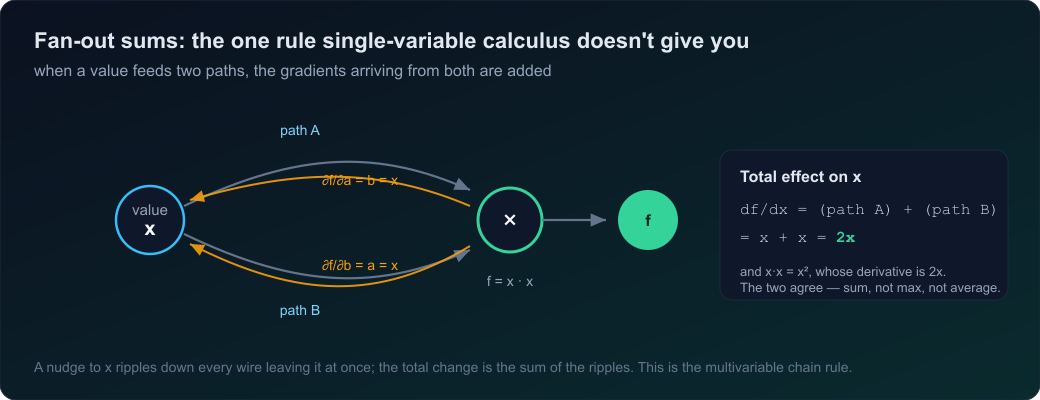
Each path gives a partial: ∂f/∂a = b = x and ∂f/∂b = a = x. Now x reaches f through two paths, so the total effect of nudging it is the sum:
df/dx = (path a) + (path b) = x + x = 2x
Check it: x · x = x², and the power rule gives 2x. They agree. Why summed, and not the max or the average? Because nudging x by one sends a ripple down every wire leaving it, simultaneously, and the total change in f is the sum of all the ripples. This is the multivariable chain rule, and it is load-bearing in every neural network on Earth — every time a hidden value feeds several downstream neurons, its gradient is the sum of the gradients coming back from all of them.
f(w, x, b) = w·x + batw=4, x=−1, b=2. Give∇f.f(w, x) = (w·x)². Find∂f/∂w(freeze x, then chain rule), and evaluate atw=3, x=2.- Using fan-out, find
df/dxforf(x) = x · x · x. Confirm against the power rule.
Show worked answers
1.  df/dw = x = -1,  df/dx = w = 4,  df/db = 1   ->   grad f = [-1, 4, 1]
2.  freeze x:  f = (w*2)^2 = (2w)^2
    chain: outside 2(2w), inside 2  ->  df/dw = 2(2w)*2 = 8w
    at w=3:  8*3 = 24     (nudge check: 24.004 -> 24)
3.  three uses of x, three paths, each partial = x*x = x^2
    df/dx = x^2 + x^2 + x^2 = 3x^2      and  x*x*x = x^3 -> 3x^2  (match)
The payoff: how it all becomes backpropagation
You now hold the entire toolkit. Return to the diagnostic — f = (a·b + c)² — and break it into named steps so every operation has a local derivative you can write in one line:
p = a * b      p = -6      local:  dp/da = b = -3,   dp/db = a = 2
u = p + c      u = -5      local:  du/dp = 1,        du/dc = 1
f = u^2        f = 25      local:  df/du = 2u = -10
Each local derivative comes straight from Concepts 1–6: the multiply node scales by the other input, the add node copies (derivative 1), the square node gives 2u. Now the trick that makes it cheap. Instead of tracing forward from each input separately, seed a 1 at the output and sweep backward, carrying a running gradient. At each node, multiply the gradient arriving from downstream by the node’s local derivative, and pass it up:
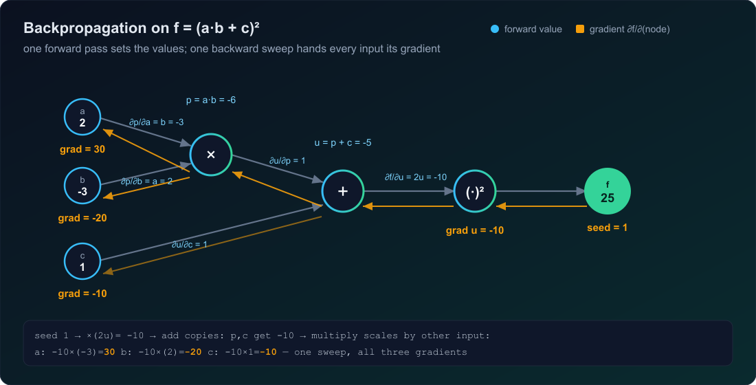
f = 25    grad = 1                          (seed:  df/df = 1)

square:   local df/du = 2u = -10
u = -5    grad = 1 * (-10) = -10

add:      local = 1, 1   (the gradient copier)
p = -6    grad = -10 * 1 = -10
c =  1    grad = -10 * 1 = -10               <- done

multiply: local dp/da = b = -3,  dp/db = a = 2
a =  2    grad = -10 * (-3) =  30            <- done
b = -3    grad = -10 * ( 2) = -20            <- done
One backward pass, all three gradients: df/da = 30, df/db = −20, df/dc = −10. Verify the first by brute force — nudge a from 2 to 2.001: p = −6.003 → u = −5.003 → f = 25.030009, and (25.030009 − 25) / 0.001 = 30.009 → 30. The analytic gradient and the numerical nudge agree, which is the only reason to trust either. That agreement — always checking your method against a nudge — is the habit that would have caught the coincidence at the very start.
And now the definition earns its weight:
Backpropagation is the chain rule applied to a computation graph, walked backward from the output, where each node multiplies the gradient arriving from downstream by its own local derivative and passes the result upstream — adding, wherever a value fanned out to more than one consumer.
Every rule in that sentence is one you just derived: multiply along a path (chain rule), each local derivative (Concepts 1–5), add at a branch (fan-out). There is nothing else in it.
From one graph to a whole neural network
A neural network is just a very long composition of functions — f(g(h(k(…)))), hundreds of layers deep, with millions of weights as inputs. To train it you need the derivative of the loss with respect to every weight. That is the chain rule, run over a composition far too long to write out by hand. Backpropagation computes it once, backward, reusing the shared sub-products instead of re-deriving the full chain for each of millions of weights — which is the only reason training a large model is feasible at all. The cost is one forward pass and one backward pass per step, no matter how many weights.
If you read How Neural Networks Learn, this is the calculus underneath the “blame” that swept backward through that network. The blame number each neuron passed back was its gradient; the rule that it multiplied by the connecting weight was the chain rule; the rule that a neuron feeding several others summed the blame coming back was fan-out. Same algorithm, now with the mathematics showing.
Where this goes next
What you have is the ~15% of calculus that scalar backpropagation actually runs on: the nudge ratio, the power rule, the chain rule, partial derivatives, the gradient, and fan-out sums. That is genuinely enough to understand the backward pass. The rest arrives on demand, when a specific thing forces it:
- eₓ and ln x — the two transcendental functions that softmax, cross-entropy, and sigmoid are built from. Two facts:
d/dx eₓ = eₓandd/dx ln x = 1/x. - Product and quotient rules — needed to derive the sigmoid and tanh gradients yourself. Mechanical; an afternoon.
- Jacobians and matrix calculus — a real layer is vector-in, vector-out, so the derivative becomes a matrix. This is the genuine wall, and it is where most self-taught practitioners stall. It is also the bridge to how frameworks like PyTorch vectorize the exact sweep you just did by hand.
You do not need any of that to start. Items above arrive when softmax or a matrix layer forces them — which is exactly the right time to learn them, and no earlier. For the wider map of what to study to go deep on AI, see the skills to learn in 2026.
- A derivative is a nudge ratio: rise over run between two points
hapart, then shrinkh. Every rule comes from that one limit. - The power rule
xⁿ → n·xⁿ⁻¹is a count of slots, not a decree — and constants have zero slope, so they die. - The chain rule multiplies local rates along a path. You never divide; division runs a rate backwards.
- Partial derivatives freeze every variable but one; the gradient is just the stack of partials.
- Fan-out sums is the one genuinely new rule: a value used many times collects the sum of the gradients from all its paths.
- Backpropagation is exactly these rules run backward over a computation graph — and a neural network is one very large such graph.
- Always verify an analytic gradient against a numerical nudge. A right answer from a wrong method is a trap waiting to spring.
Frequently asked questions
What calculus do you actually need for backpropagation?
Less than a first calculus course — roughly its most useful fifteen percent: the limit definition of a derivative, the power rule, differentiating sums and constants, the chain rule, partial derivatives, and the multivariable rule that gradients sum at a fan-out. You do not need integration, limits as a rigorous subject, or most of a standard syllabus. Softmax and matrix layers later require eₓ, ln x, and Jacobians, but scalar backpropagation runs on the short list above.
Why is the chain rule multiplication and not division?
Because derivatives compose like exchange rates. If one unit of a buys three units of u, and one unit of u buys two units of f, then one unit of a buys 3×2 = 6 units of f. You multiply the rates along the path. Dividing would be running a rate backwards, which is why the common error of “take the outer derivative and divide by the input” produces wrong gradients.
What is the derivative of a·b with respect to a?
It is b — the other input — not a·b divided by a. Derive it from the definition: nudge a by h, and (a+h)·b − a·b = h·b, so the ratio is b. The a cancels out entirely; there is nothing left to divide by. This is why the multiply node in backpropagation scales the incoming gradient by the value of the other input.
Why do gradients sum when a value is used more than once?
Because nudging that value sends a change down every wire leaving it, simultaneously, and the total effect on the output is the sum of all those separate effects. This is the multivariable chain rule. In a network, whenever a neuron’s output feeds several downstream neurons, its gradient is the sum of the gradients arriving back from each of them — not the maximum, not the average, the sum.
Is backpropagation the same as the chain rule?
Essentially yes, plus bookkeeping. Backpropagation is the chain rule applied to a computation graph and walked backward from the loss, so that each node multiplies the incoming gradient by its local derivative (and sums at fan-outs). The extra idea is efficiency: rather than re-deriving the full chain for each of millions of weights, it computes the shared sub-products once, in a single backward sweep.
How do I verify that a gradient is correct?
Nudge the input by a tiny h and measure the change in the output: [f(x+h) − f(x)] / h should match your analytic derivative. The two-sided version, [f(x+h) − f(x−h)] / (2h), is more accurate because its error shrinks with h² rather than h. This finite-difference check is the cheapest defense against being confidently wrong, and it is the habit that catches a right-answer-by-coincidence before it costs you.
Do I need to understand this to use PyTorch or TensorFlow?
To ship a model, no — the framework computes gradients for you with automatic differentiation. To debug one, reason about vanishing gradients, or defend why a model behaves as it does, yes. Autograd is doing exactly the backward sweep in this article, at scale; understanding the sweep is what lets you read what the framework is doing instead of trusting it blindly.
Educational walkthrough. Numbers are kept tiny so every step is checkable by hand; the same rules run unchanged over millions of parameters in a real network. Further reading: 3Blue1Brown’s Essence of Calculus, Andrej Karpathy’s micrograd, the Stanford CS231n notes on backprop, and Michael Nielsen’s chapter on the backpropagation algorithm.
