
Every explanation of multi-head attention eventually says that each head learns a different kind of relationship, and then moves on. That is true, and it explains nothing. It describes the outcome and skips the mechanism that forces the outcome to exist.
The mechanism is one line of arithmetic: a softmax must sum to exactly 1.0. The 64, the 128, the reshape, grouped-query attention, and the size of the KV cache that limits how many users fit on your GPU all fall out of that single constraint.
By the end you will be able to say what a head is at the level of memory layout, what the 128 numbers a head emits actually contain, and how many bytes per token the design costs you. Every number here is small enough to check by hand.
Part 3 walked the ten steps of a transformer block and left step 5, the attention computation itself, as a black box. This opens it.

- Part 1. How an LLM Answers a Question: The Complete Inference Path
- Part 2. Byte-Pair Encoding Explained: How LLMs Turn Text Into Tokens
- Part 3. Inside One Transformer Block: The Residual Stream and Its Seven Matrices
- Part 4. Multi-Head Attention Explained: Why 64 Heads Instead of One (you are here)
- Part 5. The Output Projection: How 64 Attention Heads Become One Thought
- Part 6. The Feed-Forward Network: Where a Transformer Keeps What It Knows
- Part 7. Mixture of Experts Explained: Conditional Computation From Zero
- Part 8. Attention Is All You Need, Dissected: The 2017 Figure, Box by Box
- Part 9. The Roofline Model: Why LLM Decode Is Memory-Bound
- Part 10. Continuous Batching and PagedAttention: How vLLM Keeps a GPU Busy
- Part 11. Benchmark Your Own LLM Serving Stack: Two Measurements, One Afternoon
Attention returns a blend
Definition
Attention
An operation that produces one weight per previous token saying how much of that token to take, then returns the weighted sum of what those tokens carry. It searches nothing and selects nothing.
Origin: introduced by Bahdanau and colleagues in 2014 for machine translation, where a fixed-length sentence vector was losing information on long sentences. The fix was to let the decoder look back at all encoder positions and weight them. The 2017 transformer paper kept the mechanism and deleted the recurrence around it.
Why it matters: the search metaphor predicts a winner and a lookup. The blend metaphor predicts a mixture, which is what actually comes out, and it is the only way the rest of this article makes sense.
Take the traced prompt for this series, “What is a quadratic equation?”, which tokenizes to seven tokens. The last one is ?, at position 6, and it is about to produce the first token of the answer. If its weights come out as 0.48 on equation and 0.35 on quad, the result is 0.48 of what equation carries plus 0.35 of what quad carries, plus small remainders. One vector out, and nothing won.
Section takeaways
- Attention returns a weighted mixture of what earlier tokens carry, so no token is ever selected.
- It was invented in 2014 to stop long sentences from being crushed into one fixed-length vector.
- The weights are proportions of a whole, which is the property the entire rest of the design is built on.
The constraint that causes everything
Definition
Softmax
A function that turns any list of real-valued scores into positive numbers summing to exactly 1.0, by exponentiating each score and dividing by the total. Larger gaps between scores become larger ratios between weights.
Origin: the same formula as the Boltzmann distribution in statistical physics, adopted into neural networks in the late 1980s (the name is due to John Bridle) as a way to make a network’s raw output scores behave like a probability distribution that could be trained with a likelihood objective.
Why it matters: the sum-to-one property is not decoration. It is the constraint that makes a single attention operation able to express exactly one pattern of where to look, and therefore the reason heads exist at all.
Treat one attention operation as a fixed budget. You have 1.00 to spend across the previous tokens, you must spend all of it, and you cannot spend more. Give more to one token and you have taken it from another.
Analogy
It is a budget of exactly one dollar, allocated across every token in the context. Funding one line item more means funding another less, and the books must balance to the cent every time.
Where it breaks: a real budget can be underspent or carried over. This one must be spent in full on every single attention operation, and no allocation can be negative, which is why a head with nothing useful to attend to still has to put its dollar somewhere.
Neither way of spending one budget works
Suppose ? genuinely needs three different things at once: the modifier quad, the head noun equation, and the token immediately before it for grammatical continuity.
Share the budget fairly and each need gets about 0.33, so all three arrive at a third strength and the retrieved content is a muddy average of three unrelated things. Concentrate the budget and one need arrives at 0.88 while the other two vanish. There is no third setting. The allocation strategy is not the problem. Having one budget is.
Why a wider head does not fix it
The obvious response is to give the head more room, so if 128 numbers per vector is cramped, use 8,192. It changes nothing that matters. Width affects how precisely a head can judge similarity, since a longer vector encodes finer distinctions before the dot product collapses it to one number. Width does not affect how many percentages come out. A softmax over 8,192-dimensional vectors produces one set of weights summing to 1.00, exactly like a softmax over 128-dimensional ones. The scarce resource is softmaxes, and dimensions are not scarce at all.
Section takeaways
- Softmax forces attention weights to sum to exactly 1.0, so one attention operation carries one pattern of where to look.
- A token needing three things at once gets either three diluted thirds or one need at full strength and two starved.
- Widening the vectors buys sharper judgement inside one distribution and cannot produce a second distribution.
- The scarce resource in attention is the number of softmaxes, which is what the next section buys more of.
The fix is more budgets, and they are free
Definition
Attention head
One slice of the query, key and value vectors, here 128 of the 8,192 numbers, with its own dot products, its own scores and its own softmax. Sixty-four slices means sixty-four independent budgets of 1.00 spent at the same time.
Origin: introduced in the 2017 transformer paper, whose stated reason was that a single attention operation averages away information that several attentions could keep separate. The paper used 8 heads of 64 dimensions.
Why it matters: heads add softmaxes and add nothing else. They do not add width, parameters or arithmetic, which is why the design was adopted so quickly and so universally.
One slice can put 0.92 on quad while another puts 0.88 on equation, and neither competes with the other because they are spending different money.
Two slices, two opinions, worked in full
The step that usually gets skipped is why two slices of the same vectors would ever disagree, since nothing configured them to. Here is a toy version with 8 numbers instead of 8,192, split into two halves of 4, with nothing hidden.
q            =  2  1  0  1  |  1  2  1  0
k(quad)      =  2  1  0  1  |  1  0  0  1
k(equation)  =  0  1  1  0  |  0  2  1  0

head 1 reads the left four:
  q . k(quad)      =  4 + 1 + 0 + 1  =  6
  q . k(equation)  =  0 + 1 + 0 + 0  =  1

head 2 reads the right four:
  q . k(quad)      =  1 + 0 + 0 + 0  =  1
  q . k(equation)  =  0 + 4 + 1 + 0  =  5
Divide each score by the square root of the slice width, which is 2 here, and softmax the pair. Head 1 has a gap of 2.5, and e to the 2.5 is about 12.2, so the weights land at 0.92 on quad and 0.08 on equation. Head 2 has a gap of 2.0, and e squared is about 7.4, so it lands at 0.88 on equation and 0.12 on quad.
Same query, same two keys, opposite conclusions. Nobody assigned head 1 the job of tracking modifiers. The halves simply contain different numbers, so the multiplications come out different, so the scores differ, so the softmaxes differ.
Section takeaways
- Slicing the vectors gives each slice its own softmax, so 64 slices spend 64 independent budgets at once.
- Two heads disagree because their slices hold different numbers, and for no other reason. No role was assigned.
- In the worked toy example the same query and keys produce 0.92 on one token in head 1 and 0.88 on a different token in head 2.
- Heads buy simultaneous retrievals, which is the one thing extra width can never buy.
What a head actually is
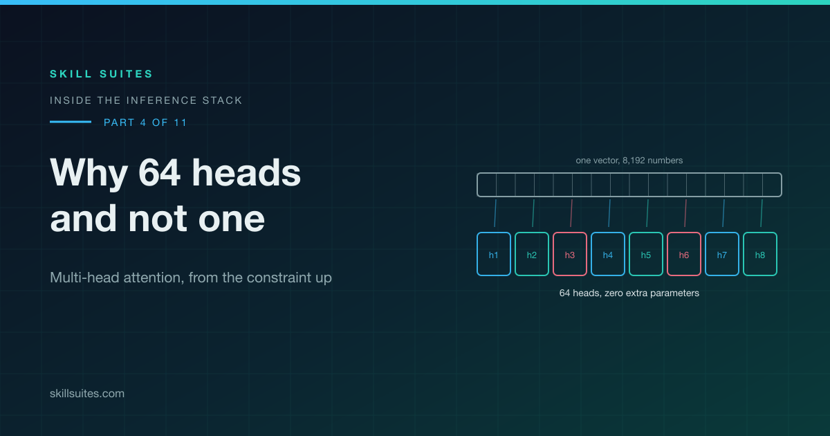
W_Q is 8,192 x 8,192 whether the model uses one head or sixty-four. It produces one vector of 8,192 numbers, and the code then reads that vector as 64 chunks of 128. Nothing is computed twice, nothing moves in memory, and creating heads is a reshape, which is to say an indexing decision, which is to say no arithmetic at all.
Analogy
One shelf holding 8,192 books, read as 64 shelves of 128. No book is moved, no book is copied, and the only thing that changed is where you agree the shelf boundaries are.
Where it breaks: a shelf boundary is a label you can move at will. This one is fixed for the entire training run, and that permanence is exactly what makes the heads specialise.
Definition
head_dim
d_model divided by the number of heads, so 8,192 over 64 gives 128. It is a consequence of the split rather than a hyperparameter anyone tuned, and it is why 64 head outputs concatenate back to exactly d_model.
Why it matters: heads cost zero extra parameters and zero extra FLOPs, so multi-head attention bought 64 simultaneous retrievals for the price of one matrix multiply. That is the trade that made it universal.
Sixty-four private worlds
Once the reshape has happened, head 3’s query only ever meets head 3’s keys. There is no path between slices, because a dot product multiplies matching positions and matching positions live in the same slice by definition. Sixty-four separate attention computations run in parallel, each inside its own 128-dimensional space, none aware that the others exist.
What is inside a head’s 128 numbers
A head returns 128 numbers, and those numbers are not a score, not an opinion about which token won, and not a probability. The weights 0.520, 0.316, 0.078 were computed, used to scale the value vectors, and thrown away. Nothing downstream can recover them.
What remains is the retrieved content: a blend of what the attended tokens carry, mixed in those proportions. In words, the head output says something like “mostly what quad carries, plus a good amount of ratic“. If a head only had to report a choice, one number would do and nothing would have been retrieved. Its job is to bring back meaning, and meaning takes 128 numbers for the same reason a token needs 8,192.
Where heads live, and where they do not
Map heads onto the ten steps of the block from Part 3 and they occupy a narrow band. They are born at step 2, when the output of W_Q, W_K and W_V is reshaped. They survive RoPE at step 3, the cache write at step 4, and attention at step 5. They are killed at step 6, when W_O concatenates and mixes them into a flat vector.
That is five of ten steps. The normalisation before them does not know about heads, the residual add after them does not, and the feed-forward network has never heard of them. Head structure belongs to the attention branch alone, never to the block and never to the residual stream.
Section takeaways
- A head is a slice of an existing vector, so heads cost zero parameters and zero FLOPs to create.
head_dim128 is 8,192 divided by 64, which is also why 64 outputs concatenate back to exactlyd_model.- Slices never interact, because a dot product only ever multiplies matching positions.
- A head emits 128 numbers of retrieved content, and the weights that produced them are discarded immediately.
- Head structure exists for 5 of the block’s 10 steps and is invisible to the rest of the model.
The partition is imposed rather than discovered
The natural assumption is that the slices correspond to something. They do not, at least not to begin with. Before training the numbers are random and dimension 0 has no relationship to dimension 1. The boundary at 128 is arbitrary. Put it at 100 or 200, or permute which dimensions belong to which head, and nothing changes. The partition is drawn through noise.
The trick is the last clause. Head 3 gets dimensions 256 to 383 on every example, at every step, for the entire training run, and only same-slice dimensions ever meet in a dot product. That fixes a rule on the model: information that needs to be compared must live in the same slice, because there is no other route for it to interact.
Meanwhile W_Q is learned and can route any input feature to any output dimension. The routing is free and the boundaries are not, so gradient descent bends the routing to fit the boundaries. Over trillions of tokens the heads differentiate, because two heads doing the same job wastes a softmax and the loss goes down when they divide the work instead.
Analogy
The walls are fixed and the furniture moves. Nobody decides what room 3 is for. The walls simply never move, so whatever ends up needing to be near itself gets carried into the same room.
Where it breaks: furniture is moved deliberately by someone with a plan. Here it is moved by gradient descent reducing a loss, so the resulting arrangement is legible only sometimes and by accident.
Definition
Induction head
A head that finds an earlier occurrence of the current token, looks at what followed it, and predicts that same continuation. Seeing A then B earlier in the context, then seeing A again, it predicts B.
Origin: named in transformer interpretability work published in 2021 and 2022, which traced the circuit across two layers and observed it forming at a specific point during training. It is widely believed to underlie in-context learning, which is the ability to pick up a pattern from the prompt with no weight updates.
Why it matters: it is direct evidence that specialisation is real rather than a story told after the fact, and it is one of the few head roles with a mechanism anyone can state precisely.
Interpretability research has named a few other results. Previous-token heads attend to position n minus 1 and nothing else. Attention sinks park spare probability mass on token 1, because softmax must sum to 1 and needs somewhere to put the remainder when a head has nothing to retrieve. Most heads have no clean description at all.
Section takeaways
- Head boundaries are drawn through random numbers at initialisation and carry no meaning at that point.
- The boundaries never move, and only same-slice dimensions can meet in a dot product, which makes the partition a hard constraint.
W_Qis learnable, so training routes features into whichever slice needs to compare them.- Specialisation happens because duplicated heads waste a softmax, so the loss falls when heads divide the work.
- Induction heads, previous-token heads and attention sinks are named examples, and most heads have no clean description.
The single-head counterfactual saves nothing
If heads are free, the reverse question is worth asking. Setting n_heads to 1 means head_dim becomes 8,192: one query vector 8,192 long, one key vector 8,192 long, one attention distribution per token per layer.
Most people assume that must be cheaper. Parameters, KV cache and FLOPs are all identical to 64-head attention, because every one of those costs depends on total width and total width is unchanged. One head of 8,192 dimensions and 64 heads of 128 are the same 8,192 numbers. The attention FLOPs for our seven tokens come to 7 x 7 x 8,192 x 1 in one case and 7 x 7 x 128 x 64 in the other, the same product.
Single-head is dominated rather than a tradeoff. You pay the same and receive one distribution instead of sixty-four.
Definition
MQA and GQA
Multi-query attention keeps all 64 query heads and shares a single key/value head between them. Grouped-query attention is the middle setting: 64 query heads sharing 8 key/value heads, one per group of eight.
Origin: MQA was introduced by Noam Shazeer in 2019 in “Fast Transformer Decoding”, which identified the KV cache as the thing that makes decoding memory-bound and cut it by sharing one write head. It lost measurable quality, so GQA followed in 2023 as the interpolation that keeps most of the saving and recovers the quality, including a recipe for converting existing multi-head checkpoints rather than retraining from scratch.
Why it matters: cutting query heads costs quality and saves nothing. Cutting key/value heads costs almost no quality and saves enormously. That asymmetry is the entire reason GQA exists and single-head does not.
| Configuration | Query heads | KV heads | Params vs MHA, per layer | KV cache, bytes per token per layer | Quality |
|---|---|---|---|---|---|
Single head, head_dim 8192 |
1 | 1 | identical | 32,768 | worst |
| MHA, 64 heads of 128 | 64 | 64 | baseline | 32,768 | best of the four |
| GQA, groups of 8 | 64 | 8 | 224 MB smaller | 4,096 | close to MHA |
| MQA, one shared KV head | 64 | 1 | 252 MB smaller | 512 | measurably below MHA |
The parameter column is straightforward to derive. Under MHA, W_K and W_V are each 8,192 x 8,192, which is 128 MB apiece in bf16. Under GQA they are 8,192 x 1,024, or 16 MB apiece, saving 224 MB per layer across the two. Under MQA they are 8,192 x 128, or 2 MB apiece, saving 252 MB. W_Q and W_O never change size in any of these variants.
Why not 512 heads, then
Because head_dim equals d_model divided by n_heads, so more heads means thinner heads. At 512 heads each would get 16 dimensions, and a 16-dimensional space cannot hold many nearly orthogonal directions, so the query goes blunt and its distribution uninformative. Quality degrades in both directions from the middle.
In practice
A head_dim near 128 is close to universal across model families, and it also suits GPU tile sizes well. If you are choosing head counts for a model of your own, pick the count that lands head_dim in the 64 to 128 range and treat anything outside it as a claim you need to justify with measurements.
One honest footnote. Pruning research has shown that many heads can be removed from a trained model with little quality loss. That is a statement about the finished model rather than about how to build one, because training with a single head from the start produces a clearly worse one. The redundancy appears to be needed during learning, so that useful specialisations have somewhere to form.
Section takeaways
- A single-head model has identical parameters, identical cache and identical FLOPs, and returns one distribution instead of 64.
- Cutting query heads is pure loss. Cutting key/value heads is where all the savings are.
- GQA cuts per-layer cache from 32,768 bytes per token to 4,096 and saves 224 MB of weights per layer.
- MQA cuts cache to 512 bytes per token and gives up measurable quality, which is why GQA became the default.
- More heads means thinner heads, and below roughly 64 dimensions a head’s query goes blunt.
The eight phases, traced on one token
Now run the whole branch on the ? at position 6, with the running model: d_model 8,192, 64 query heads, 8 KV heads, head_dim 128, 80 layers.
Arrival and normalise
The block begins with seven token vectors of 8,192 numbers each. There is no q, no k, no v, no head structure. A copy of the vector is rescaled by RMSNorm so its numbers sit in a controlled range, and the residual stream itself is untouched, waiting for the add at the end.
Project: three matrices, three different widths
The normalised copy is multiplied by three learned matrices in parallel. All three read the same input and produce different results. The widths differ because this model uses grouped-query attention: q comes out 8,192 wide, while k and v come out only 1,024 wide. That is not a compression step. W_K and W_V are physically smaller matrices.
Reshape, and which query head reads which keys
The 8,192 numbers of q are read as 64 groups of 128. The 1,024 numbers of k and v are read as 8 groups of 128. Both close exactly, and this is the moment heads begin to exist. With 64 query heads and only 8 KV heads, they are matched in groups of eight: query heads 1 to 8 all read KV head 1, query heads 9 to 16 read KV head 2, and so on. Sixty-four different questions, asked of eight shared sets of material.
Cache append
Definition
KV cache
The stored key and value vectors for every token seen so far, kept per layer so that a decode step does not have to recompute them. Only the 8 KV heads are stored, since q is consumed in this step and discarded.
Origin: it became standard as soon as decoder-only transformers were served autoregressively, because without it generating token n would mean recomputing the keys and values for all n minus 1 earlier tokens on every single step, turning linear work into quadratic work.
Why it matters: caching q would be pointless and caching k and v is mandatory, which is exactly why GQA shrinks W_K and W_V and leaves W_Q alone.
Score, scale and mask
Inside head 7, take this token’s q and multiply it against the k of every position, summing 128 products each time. Seven positions give seven raw numbers: say 14, 9, 6, 46, 41, 25, 11. They are large because each is a sum of 128 terms.
Divide every score by the square root of 128, about 11.3, giving 1.2, 0.8, 0.5, 4.1, 3.6, 2.2, 1.0. Then set any score for a future position to minus infinity so it vanishes under the exponential. Our token is last, so nothing is masked here. For the token at position 2, positions 3 through 6 would be blanked.
Definition
Causal mask
Setting the score for every future position to minus infinity before the softmax, so those weights come out as exactly zero. Position 2 can see positions 0, 1 and 2, and nothing after.
Origin: part of the decoder in the 2017 transformer paper. It exists so that the model can be trained on every position of a sequence in one parallel pass while still being forced to predict each token from its left context only. Without it the model would see the answer it is being asked to predict.
Why it matters: it is the reason prefill can process your whole prompt in one shot and decode cannot. Every token’s view is fixed and never widens, which is what makes the KV cache valid to reuse.
Why the divisor is the square root of the head dimension
Definition
Scaled dot-product attention
Attention with every score divided by the square root of head_dim, so 11.3 here, before the softmax runs.
Origin: the 2017 transformer paper added the divisor after observing that for large head dimensions the raw dot products grow large in magnitude, pushing softmax into regions where its gradient is almost zero. The scaling was adopted to fix a training problem rather than an accuracy problem.
Why it matters: the divisor tracks head_dim and not d_model. This is one of very few places in the whole branch where the head count changes the arithmetic instead of only the bookkeeping.
Treat the entries of q and k as roughly independent with zero mean and unit variance. Their dot product is a sum of 128 such products, so it has variance 128 and a standard deviation of about 11.3. Scores therefore arrive spread over a range that grows with the square root of the head dimension, purely as an artefact of how many terms were summed.
Softmax cares about differences and it exponentiates them. Leave the scores unscaled and the gap between 46 and 41 becomes e to the 5, about 148, so quad receives roughly 148 times the weight of ratic and every other position rounds to zero. Attention degenerates into a hard argmax and stops producing blends. Worse for training, the softmax gradient is proportional to p times 1 minus p, which collapses to zero once a weight saturates near 1.0, so no learning signal flows back. Scaled, the gap of 0.5 becomes e to the 0.5, about 1.65, and quad lands at 0.520 against ratic at 0.316. That ratio is 1.65, so the arithmetic checks.
Softmax and blend
Softmax turns the seven scaled scores into seven weights that sum to exactly 1.000: 0.029, 0.019, 0.014, 0.520, 0.316, 0.078, 0.023. Head 7 has decided, in whatever sense a head decides anything, that it wants mostly quad.
Then multiply each position’s v vector by its weight and add them all together. Out comes 128 numbers, and that is head 7’s complete and finished output for this token.
Concatenate, mix, add
All 64 heads ran the identical sequence on their own slices, at the same time, with no awareness of each other. Their outputs are concatenated, placed end to end in fixed slots. Head 1 occupies positions 0 to 127, head 7 occupies 768 to 895, and every head keeps all 128 of its numbers. Nothing is compared, nothing wins, nothing is discarded. 64 times 128 is 8,192, so the pieces form one vector of exactly the width we started with.
At this instant the findings sit in 64 sealed compartments that have never interacted. W_O, an 8,192 x 8,192 matrix, dissolves them: every output number is a weighted sum of all 8,192 inputs, so the sum runs straight across the compartment boundaries and any head’s finding can land anywhere. After that multiply, no individual head output exists in memory. Only its influence survives, blended into the result, which is added to the residual stream that has been waiting since the start of the block. The branch is over.
That output projection deserves its own article, and it gets one in Part 5, on how 64 attention heads become one thought.
Every tensor in the branch, with its shape
Shapes are for the seven-token prefill, one layer, bf16, at two bytes per number. Reading down the size column shows where the memory actually goes, which is almost entirely into the 8,192-wide tensors.
| Tensor | Shape | Size | Note |
|---|---|---|---|
x |
7 x 8192 | 112 KB | residual stream in, one vector per token |
x_norm |
7 x 8192 | 112 KB | rescaled copy, used only inside the branch |
q flat |
7 x 8192 | 112 KB | output of W_Q, no heads yet |
k flat |
7 x 1024 | 14 KB | output of W_K, eight times narrower |
v flat |
7 x 1024 | 14 KB | output of W_V |
q reshaped |
7 x 64 x 128 | 112 KB | same memory, reinterpreted |
k, v reshaped |
7 x 8 x 128 each | 14 KB each | same memory, reinterpreted |
| K cache slice | 7 x 8 x 128 | 14 KB | this layer, persists across decode steps |
| V cache slice | 7 x 8 x 128 | 14 KB | this layer, persists across decode steps |
| scores | 64 x 7 x 7 | 6 KB | one raw number per head per query per key |
| weights | 64 x 7 x 7 | 6 KB | after scaling, masking and softmax |
| head outputs | 7 x 64 x 128 | 112 KB | 64 vectors of 128 per token |
concat |
7 x 8192 | 112 KB | the same buffer, read flat again |
attn_out |
7 x 8192 | 112 KB | after W_O, no head structure left |
x' |
7 x 8192 | 112 KB | residual stream out |
In at 8,192 and out at 8,192. Seven tokens in and seven tokens out. Only the shape of each token’s vector changes, and it changes back.
Section takeaways
- The branch is eight phases: normalise, project, reshape, cache, score, scale and mask, softmax and blend, then concatenate and mix.
- Under GQA the q projection is 8,192 wide while k and v are 1,024, and only the 8 KV heads are cached.
- The causal mask blanks future positions before the softmax, which is what makes the cached entries valid to reuse forever.
- The square root of 128 divisor was adopted to stop softmax saturating and killing the gradient, and it tracks
head_dim. - Every tensor enters and leaves at 8,192 wide. The head structure exists only between the reshape and
W_O.
The KV cache arithmetic that decides your concurrency
This is the number that determines how many people can share one GPU. Per token, per layer, under grouped-query attention:
2 tensors (k and v) x 8 KV heads x 128 dims x 2 bytes  =  4,096 bytes
across 80 layers                                       =  327,680 bytes  =  320 KB per token
The same model with full multi-head attention, meaning 64 KV heads rather than 8:
2 x 64 x 128 x 2  =  32,768 bytes per layer
across 80 layers  =  2,621,440 bytes  =  2.5 MB per token
Eight times more, for the same weights, the same FLOPs, and quality that measures within noise of full MHA. An 8,192-token conversation carries 2.5 GB of cache under GQA and 20 GB under MHA. This model is about 140 GB of bf16 weights, so it already spans a multi-GPU node. On an eight-way 80 GB node that is 640 GB total, leaving roughly 500 GB after weights and activation workspace. Divide it out: GQA fits about 200 concurrent 8K conversations, and MHA fits about 25.
In practice
Concurrency is cache capacity divided by cache per conversation, so size it directly: (total GPU memory, minus weights, minus activation workspace) divided by (320 KB times your median conversation length in tokens). If that number comes out below your expected concurrent users, no amount of batching tuning will save you and the fix is a smaller model, a shorter context or more GPUs.
That ratio is why grouped-query attention appeared in every serious open-weight model within about a year of the paper. It is also why the rest of this series keeps returning to the KV cache: it is read in full on every decode step, so it is a bandwidth problem as well as a capacity problem. Part 9 shows why that makes decode memory-bound, and Part 10 covers how vLLM pages the cache so that the 200 is achievable rather than theoretical. The same arithmetic drives the decision to move LLM workloads on-prem, and the piece on latency, throughput and queueing covers what happens once those 200 slots start filling up.
Section takeaways
- GQA costs 4,096 bytes per token per layer, which is 320 KB per token across all 80 layers.
- Full MHA costs 32,768 bytes per layer and 2.5 MB per token, eight times more for the same weights and FLOPs.
- An 8K conversation is 2.5 GB of cache under GQA and 20 GB under MHA.
- On an eight-way 80 GB node that is roughly 200 concurrent conversations against roughly 25.
- The cache is read in full on every decode step, so it is a bandwidth problem as well as a capacity problem.
Key takeaways
- A softmax sums to 1.0, so one attention operation expresses exactly one pattern of where to look. Multi-head attention exists to buy more of those patterns.
- Widening a head buys precision within one distribution and cannot buy a second one. The scarce resource is softmaxes, not dimensions.
- A head is a slice, not a matrix.
W_Qis 8,192 x 8,192 at any head count, so heads cost zero parameters and zero FLOPs to create. - A head returns 128 numbers of retrieved content. The weights that produced them are discarded, so nothing downstream can compare heads.
- The partition is imposed on random numbers, not discovered in them. Specialisation appears because the boundaries never move and the routing into them is learned.
- A single-head model has identical parameters, cache and FLOPs, with one distribution instead of sixty-four. It is dominated rather than a tradeoff.
- Cutting KV heads is the only change here that saves memory. GQA costs 320 KB per token against 2.5 MB for MHA, an eight times difference in concurrency.
Frequently asked questions
Why does multi-head attention use 64 heads instead of one wide head?
Because a softmax must sum to exactly 1.0, so one attention operation can express only one pattern of where to look. Sixty-four heads means sixty-four independent budgets of 1.0 spent at the same time without competing, and a token that needs three different things from three different places can get all three at full strength.
Do attention heads add parameters to a transformer?
No. W_Q, W_K, W_V and W_O have the same shapes whether the model uses 1 head or 64. Heads are created by reshaping the projection output into groups, which is an indexing decision with no arithmetic and no data movement.
Why is the attention score divided by the square root of the head dimension?
A dot product of two 128-dimensional vectors is a sum of 128 terms, so its standard deviation grows like the square root of 128, about 11.3. Without the divisor, softmax exponentiates gaps that are roughly 11 times too large, saturates to a hard argmax, and its gradient collapses to zero so training stalls.
What is the difference between MHA, MQA and GQA?
All three keep 64 query heads. Multi-head attention gives each query head its own key and value head, multi-query attention shares a single KV head across all of them, and grouped-query attention shares one KV head per group of eight. Only the material being searched is shared, never the questions being asked.
How much KV cache does grouped-query attention save?
On a 70B-class model with 80 layers, 8 KV heads and head_dim 128, the cache is 2 x 8 x 128 x 2 bytes per layer, which is 320 KB per token across all layers. Full multi-head attention with 64 KV heads would cost 2.5 MB per token, so GQA is eight times smaller and fits roughly eight times as many concurrent conversations.
Can you remove attention heads from a trained model?
Often yes. Pruning studies have found that many heads can be dropped from a trained model with little quality loss. That does not mean you can train with fewer heads, because a model trained with one head from the start is clearly worse. The redundancy appears to matter during learning rather than at inference.
Sources and further reading
- Attention Is All You Need, the original multi-head attention formulation, including the scaled dot product and the ablation on head count.
- Neural Machine Translation by Jointly Learning to Align and Translate, Bahdanau et al., where attention was introduced in 2014.
- Fast Transformer Decoding: One Write-Head is All You Need, the multi-query attention paper, which frames the KV cache as the decode bottleneck.
- GQA: Training Generalized Multi-Query Transformer Layers from Multi-Head Checkpoints, the grouped-query attention paper and its quality comparisons.
- Are Sixteen Heads Really Better than One?, the head pruning result behind the honest footnote above.
- RoFormer: Enhanced Transformer with Rotary Position Embedding, the RoPE step applied per head between the reshape and the cache write.
- vLLM documentation, for how the KV cache arithmetic here turns into real concurrency limits on real hardware.
Check your understanding
Take the 15 question quiz on this article
The same 15 questions every time, picked to cover every idea this article teaches, out of 30 written for it. The order of the questions and the order of the answer choices reshuffle on every attempt, so a retake never looks identical to the last one. It runs here on the page and keeps your place, so you can go and read a section and come back without losing anything. You get a full report at the end: your score, the correct answer to anything you missed, why it is correct, and a link straight back to the section it came from.
- 15 questions
- same set every time
- 8 knowledge areas
- hint on every question
- timed, no limit
