
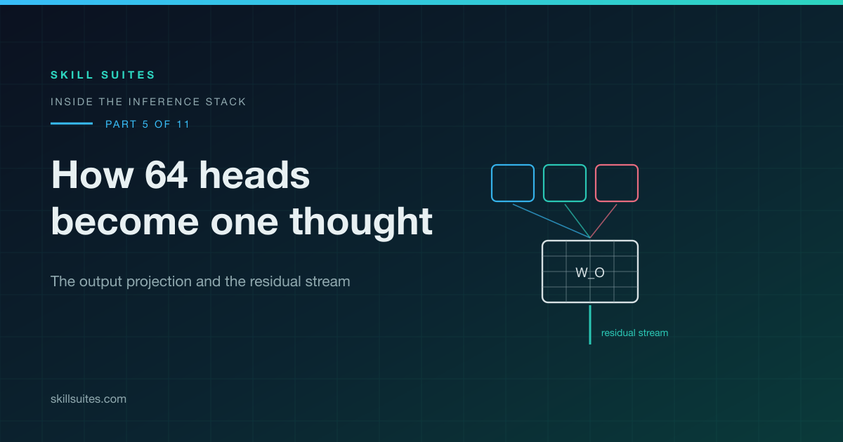
Sixty-four attention heads have just finished work. Each produced 128 numbers, and not one of them knows what the other sixty-three found. The output projection, the matrix written W_O, is the operation that fixes that. It is also the least explained matrix in the block, usually waved through as “concatenate the heads and project”.
This article does two things. First it works a complete output projection by hand, on a toy small enough to check with a pen: 3 heads of 2 numbers each, and a 6 x 6 grid of weights. Every number below is checkable. Second it follows the result out of the block and into the residual stream, and shows why one addition sign fixes the width of the model at 8,192 for all 80 layers.
The running model is the one used throughout the series and in the previous part on why 64 heads beat one: 80 layers, d_model 8,192, 64 query heads, 8 key/value heads, head_dim 128.
- Part 1. How an LLM Answers a Question: The Complete Inference Path
- Part 2. Byte-Pair Encoding Explained: How LLMs Turn Text Into Tokens
- Part 3. Inside One Transformer Block: The Residual Stream and Its Seven Matrices
- Part 4. Multi-Head Attention Explained: Why 64 Heads Instead of One
- Part 5. The Output Projection: How 64 Attention Heads Become One Thought (you are here)
- Part 6. The Feed-Forward Network: Where a Transformer Keeps What It Knows
- Part 7. Mixture of Experts Explained: Conditional Computation From Zero
- Part 8. Attention Is All You Need, Dissected: The 2017 Figure, Box by Box
- Part 9. The Roofline Model: Why LLM Decode Is Memory-Bound
- Part 10. Continuous Batching and PagedAttention: How vLLM Keeps a GPU Busy
- Part 11. Benchmark Your Own LLM Serving Stack: Two Measurements, One Afternoon
Where we are: 64 sealed boxes
Definition

Output projection (W_O)
The 8,192 x 8,192 matrix that multiplies the concatenated head outputs and produces the single vector the attention branch contributes to the residual stream.
Origin: it arrived with multi-head attention in the 2017 transformer paper, written W^O there. It exists because splitting attention into heads leaves you with 64 separate results and the block is contractually required to return one vector of exactly d_model numbers. Something has to put the pieces back together, and that something also turned out to be where most of the useful work happens.
Why it matters: it is the only path by which any two heads can ever influence each other. Remove it and multi-head attention degenerates into 64 unrelated operations sharing a container.
Attention has run and each of the 64 heads produced 128 numbers. Lay them side by side and you have 8,192 numbers again, one vector, the same width as the thing that went in.
It is not one vector in any useful sense. Numbers 0 to 127 came from head 1, numbers 128 to 255 came from head 2, and they are neighbours in memory that have never influenced each other, not once. Adjacency is not communication, which is a distinction worth internalising well beyond transformers if you spend time reading memory layouts for a living.
Here is why that matters. Say head 1 found “this is a definition question” and head 23 found “the important noun is equation”. Both findings are real, both are correct, and neither is worth much alone. The thought the model actually needs is “define the word equation”, and that thought is a combination of the two. Right now it cannot form, because the two findings sit in different compartments and nothing connects the compartments.
Section takeaways
- Concatenated head outputs look like one 8,192-number vector and behave like 64 unrelated lists of 128.
- Head boundaries are memory adjacency and nothing more. No information has crossed them at this point.
- Two correct findings in two heads cannot combine into the conclusion the model needs without a mixing step.
W_Oexists because the block must return exactlyd_modelnumbers, and it is the only route between heads.
The multiply, worked by hand
The toy: 3 heads, 2 numbers each
Three heads have just finished. Head 1 returned 3, 1. Head 2 returned 0, 2. Head 3 returned 5, 4. Concatenated, that is the 6-number vector [3, 1, 0, 2, 5, 4], in three sealed groups of two. The real model is 64 heads of 128 numbers, giving 8,192. Same structure, bigger numbers, and no additional ideas.
W_O is a grid of weights, one column per output
Six numbers in, six numbers out, so W_O here is a 6 x 6 grid. Read it by column, because each column is the complete recipe for one output number: how much of each of the six inputs to use. Column 1 is the recipe for output 1, column 2 is a different recipe for output 2, and so on for six independent recipes over the same six inputs. In the running model there are 8,192 columns over 8,192 inputs, which is 67 million learned weights per layer.
| Input | out1 | out2 | out3 | out4 | out5 | out6 |
|---|---|---|---|---|---|---|
| in1 (head 1) | 0.5 | 0.1 | 0.0 | 0.3 | 0.0 | 0.2 |
| in2 (head 1) | 0.0 | 0.4 | 0.2 | 0.0 | 0.1 | 0.0 |
| in3 (head 2) | 0.2 | 0.0 | 0.5 | 0.1 | 0.0 | 0.3 |
| in4 (head 2) | 0.0 | 0.3 | 0.0 | 0.4 | 0.2 | 0.0 |
| in5 (head 3) | 0.8 | 0.0 | 0.1 | 0.0 | 0.6 | 0.1 |
| in6 (head 3) | 0.1 | 0.2 | 0.0 | 0.5 | 0.0 | 0.4 |
Analogy
Each column is a recipe and the six inputs are the ingredients on the bench. Output 1 takes a lot of ingredient 5, a little of 1 and 6, and none of the rest. Output 3 is a completely different dish made from the same bench.
Where it breaks: a cook chooses proportions on purpose and can taste the result. These 67 million proportions were fitted by gradient descent to reduce a loss, so most of them correspond to nothing a person would recognise as an ingredient.
Output number 1, every step
Take the input vector and column 1. Multiply matching positions, then add the six results. The six products are 3(0.5) = 1.5, then 1(0.0) = 0.0, then 0(0.2) = 0.0, then 2(0.0) = 0.0, then 5(0.8) = 4.0, then 4(0.1) = 0.4. Add them: 1.5 + 0.0 + 0.0 + 0.0 + 4.0 + 0.4 = 5.9.
Now group those products by which head they came from. Head 1 contributed 1.5, head 2 contributed 0.0, head 3 contributed 4.4. One output number, built from two heads at once.
The other five outputs
Repeat with each remaining column. Same six inputs every time, different recipe every time, so no two outputs are built the same way.
| Output | From head 1 | From head 2 | From head 3 | Total |
|---|---|---|---|---|
| out1 | 1.5 | 0.0 | 4.4 | 5.9 |
| out2 | 0.7 | 0.6 | 0.8 | 2.1 |
| out3 | 0.2 | 0.0 | 0.5 | 0.7 |
| out4 | 0.9 | 0.8 | 2.0 | 3.7 |
| out5 | 0.1 | 0.4 | 3.0 | 3.5 |
| out6 | 0.6 | 0.0 | 2.1 | 2.7 |
Head 3 dominates output 1 and is nearly absent from output 3. Head 2 is silent in outputs 1, 3 and 6. All three heads land in outputs 2 and 4. Nothing in the input said any of that, and it is entirely the grid’s doing.
Section takeaways
- The output projection is one matrix multiply and contains no separate merge step.
- Every column is an independent recipe for one output number over every input number.
- In the worked toy, output 1 is 5.9, assembled from 1.5 of head 1 and 4.4 of head 3, with head 2 contributing nothing.
- The real matrix is 8,192 columns over 8,192 inputs, which is 67 million learned weights per layer.
- Which heads reach which outputs is decided entirely by the grid and not at all by the heads.
The three jobs in one multiply
Job one: combining findings across head boundaries
Look again at where 5.9 came from. Part of it was head 1’s work and part of it was head 3’s, and the plus sign between them did not know or care that a compartment wall sat there. That is the whole of what mixing means. There is no separate merge step, the addition simply runs across the boundaries, and the boundaries mean nothing to it.
Translate that back to the real thing. Head 1 found “this is a question”. Head 3 found “the topic is equations”. Neither is actionable alone, the conjunction is, and after the multiply a single number carries something neither head knew.
The three inputs that survived their weights in that second example came from heads 1, 3 and 4. Three heads, one number, one addition.
Job two: routing, or where a finding lands
Definition
Direction, or subspace, of the residual stream
A particular combination of the 8,192 coordinates that later blocks learn to read for a particular kind of information. Writing “into a subspace” means adding a vector that points along those coordinates.
Origin: the framing was developed in transformer interpretability work published from 2021 onward, which treats the stream as a communication channel that components read from and write to, rather than as an activation to be inspected coordinate by coordinate.
Why it matters: it makes “where a finding lands” a real question with a real answer, and the answer is decided by W_O rather than by the head that produced the finding.
The weights do not only combine. They also decide where the result gets written, because the residual stream is not undifferentiated. Different directions in those 8,192 numbers end up carrying different kinds of information, since later blocks learn to read particular directions for particular things.
So the division of labour is clean. Heads decide what to look for, and the output projection decides what to do with what they found, including which part of the stream to file it in. A head that studies nouns can have its output written into whichever positions carry noun information, and it never has to know that.
Job three: a zero is a decision too
Go back to the grid and count the zeros. A zero is not an absence of a weight. It is a learned instruction to exclude one input from one output.
Output 1 is the cleanest case. Head 2’s two numbers are 0 and 2. The zero contributes nothing whatever its weight, and the 2 is switched off by a learned 0.0 in column 1. Head 2 is deliberately not heard in output 1, and that decision is made independently for all 8,192 outputs. A head can be loud in some places and silent in others, in the same layer, on the same token.
Section takeaways
- Combining is not a step. It is what happens when a sum runs across boundaries that the arithmetic cannot see.
- Routing is the second job: the weights decide which direction of the residual stream a finding is written into.
- A learned zero is an active exclusion, deciding that one head is not heard in one specific output.
- All three decisions are made independently for each of the 8,192 outputs, on every token.
- Heads decide what to look for and
W_Odecides what is done with it, including where it gets filed.
Reading the grid two ways, and why heads specialise
Read a column and you get “which heads feed this output?”. Read a row and you get “where does this head’s information go?”. The row view is the one interpretability researchers use, because a row block shows which directions of the residual stream a given head is able to write into. That is how a claim like “this head writes to the topic subspace” gets established in the first place.
The row view has a practical consequence. Because W_O multiplies a concatenation, you can slice it into 64 blocks of 128 rows, one block per head, and the block’s output is exactly the sum of the 64 per-head products. Concatenate-then-project and project-per-head-then-add are the same arithmetic. That equivalence is why it is legitimate to talk about “head 12’s contribution to the residual stream” as a thing that exists.
Now take W_O away and see what breaks. Each head’s 128 numbers would go straight onto the residual stream and stay in their own slice forever, so head 12 would occupy positions 1408 to 1535 in every block, in every layer, permanently. Nothing could ever combine two heads.
The deeper point follows from that. A head is only useful if its finding can be used, and the output projection is the only route by which it can be. During training, a head that discovers something valuable is rewarded only when W_O has learned to carry that output somewhere the rest of the model benefits from. The two co-adapt from the same gradient, so specialisation and routing develop together and neither is worth anything without the other.
Section takeaways
- Columns answer “which heads feed this output”. Rows answer “where can this head write”.
- Slicing
W_Ointo 64 row blocks and summing per-head products is identical arithmetic to one big multiply. - That equivalence is what makes “head 12’s contribution to the stream” a well defined quantity rather than a metaphor.
- Without the projection, every head would own one fixed slice of the stream for the life of the model.
- Head specialisation and output routing are learned from the same gradient and are useless separately.
The four attention matrices, by size
Put the numbers for the running model side by side, per layer, in bf16, with 64 query heads and 8 key/value heads under grouped-query attention.
| Matrix | Shape | Parameters | bf16 size | Receives |
|---|---|---|---|---|
W_Q |
8,192 x 8,192 | 67.1M | 134 MB | the normalised residual stream vector |
W_K |
8,192 x 1,024 | 8.4M | 16.8 MB | the normalised residual stream vector |
W_V |
8,192 x 1,024 | 8.4M | 16.8 MB | the normalised residual stream vector |
W_O |
8,192 x 8,192 | 67.1M | 134 MB | the 64 head outputs, concatenated |
Two things stand out. The output projection is exactly the same size as W_Q, and it is four times the size of W_K and W_V combined. It accounts for 44 percent of the attention block’s parameters.
W_K and W_V are small for a reason that has nothing to do with importance: grouped-query attention gives them 8 heads instead of 64, to shrink the KV cache. W_O is large for a reason that has everything to do with its job. It holds 8,192 separate recipes, each drawing on all 64 heads, plus the routing decision for every head into every region. That is a lot of decisions to store.
In practice
Across all 80 layers the output projections alone come to 5.4 billion parameters and about 10.7 GB of bf16 weights, which is roughly 8 percent of the whole model. When you are sizing hardware for a model you intend to host yourself, that is one line item bigger than most people’s entire fine-tuned adapter budget.
So the three jobs are combine, select and route, and they are not three steps. They are one multiply, and the same weights do all three at once.
Section takeaways
W_Ois 67.1M parameters and 134 MB in bf16, identical toW_Qand four timesW_KplusW_V.- It is 44 percent of the attention block, which is proportionate to the number of decisions it stores.
W_KandW_Vare small because of grouped-query attention, which is a cache decision and not a statement about importance.- Across 80 layers the output projections are 5.4 billion parameters and about 10.7 GB, roughly 8 percent of the model.
- Combine, select and route are three descriptions of one multiply, not three sequential operations.
Replace or add: the choice that fixes everything
The output projection has produced 8,192 numbers. The block now has to hand something to the next block, and there are exactly two options. Replace means throw away what came in and pass on the new numbers. Add means keep what came in and add the new numbers to it. Transformers add, and almost everything else about the architecture follows from that one choice, as the earlier walk through a single block set up.
Definition
Residual connection
Adding a block’s output to its input instead of replacing it, so the block computes a correction to a running total rather than a new value.
Origin: introduced by He and colleagues in 2015 for image recognition, where networks past about 20 layers were getting worse with depth, and not from overfitting. The skip connection let them train 152 layers. The transformer inherited the idea in 2017 and it is the reason an 80-layer stack is routine.
Why it matters: it is why nothing written early is ever erased, and it is also what forces every layer in the model to be exactly the same width.
What replacing would cost
Follow three blocks under replace. Block 1 notices something important, block 2 produces its own output and hands that on instead, and block 1’s finding is now unrecoverable. Not buried, not hard to reach, gone. Any block that needed block 1’s finding would have to be block 2, because block 2 is the last one that ever sees it. Eighty blocks under replacement would be eighty strangers, each able to cooperate only with its immediate neighbour.
What adding buys
The same three blocks under add. Each block’s contribution lands on a running total, nothing is destroyed, so block 30 can still read what block 3 wrote and block 71 can still read both.
Analogy
One page running the whole height of the model. Every block reads the page, writes a note on it, and passes it upward, and nobody has an eraser. It is append-only in the same sense that a log-structured storage engine is append-only, and it buys the same thing: history that later readers can still use.
Where it breaks: a log holds discrete records you can read back one at a time. The page holds a running sum, so two notes written to the same coordinates are added together and can only be separated approximately, by tools like the ones at the end of this article.
Definition
Circuit
A chain in which one block writes a partial result into the stream, a later block reads it and writes a refinement, and a later one again reads that. The chain implements a behaviour that no single component contains.
Origin: the term comes from transformer interpretability work published from 2021, which borrowed it from earlier circuits research on vision models. It was adopted because “which neuron does what” turned out to be the wrong question, and “which path carries what between components” turned out to be answerable.
Why it matters: circuits are the reason multi-step reasoning is possible inside a fixed depth, and they exist only because the stream is additive and nothing gets erased.
Section takeaways
- A block can replace the stream or add to it, and transformers add.
- Under replacement, a finding is only usable by the immediately following block and is then gone forever.
- Under addition every contribution stays in the running total, so block 71 can still read what block 3 wrote.
- The residual connection came from 2015 image models, where depth past about 20 layers was making networks worse.
- Circuits, which chain partial results across blocks, exist only because the stream is append-only.
Why the width can never change, and why 80 layers train
You cannot add two lists of different lengths. Every block adds its result to what came in, so every block must produce exactly as many numbers as it received. That is why d_model is 8,192 at every layer boundary in the model. It is not a preference, and addition demands it.
Say plainly what that rules out. You cannot taper a transformer the way you taper a convolutional network, narrowing as it goes deep. You cannot widen the later layers because they are doing harder work. You cannot insert a block that outputs 12,288 numbers between two blocks that expect 8,192. Every architectural change to the stream width has to be made once, globally, for all 80 layers, or it has to be paired with a projection that puts the width back.
The feed-forward network is the clean illustration. It widens to 28,672 and then comes back down to 8,192 before anything is added, so the wide part exists only inside the branch and never touches the page. The next part in this series works through what happens up there.
One more consequence, easier to feel than to prove. During training a correction signal has to travel from the output all the way back to block 1. Under replacement it passes through 80 transformations and gets scaled at every one, and multiplying 80 small numbers together gives a result indistinguishable from zero, so block 1 learns nothing. Under addition there is a direct path down the running total that the signal travels untouched.
What the residual stream makes visible
Definition
Logit lens and activation patching
Two ways of reading the stream mid-model. The logit lens applies the final unembedding to the stream partway up and reads off what the model would have predicted at that depth. Activation patching swaps one component’s contribution in from a second run and watches the prediction move.
Origin: the logit lens was introduced in a widely cited 2020 blog post and named for what it does. Activation patching, also called causal tracing, was developed in 2022 work on locating factual associations inside GPT models, adopted because correlational readings of activations could not distinguish a component that causes a prediction from one that merely correlates with it.
Why it matters: both techniques work only because every block adds into the same 8,192-number space, which puts an intermediate stream in the same coordinate system as the final one.
In practice
Treat the output of a logit lens or a patching experiment as evidence and not as an explanation. Both have known failure modes, particularly on models whose intermediate representations are not well aligned with the final unembedding, so a clean-looking readout can be an artefact of the tool rather than a fact about the model.
Section takeaways
- Addition requires matching widths, which is the real reason
d_modelis 8,192 at every one of the 80 layer boundaries. - You cannot taper, widen or splice a differently-shaped block into the stack without a projection that restores the width.
- The feed-forward branch widens to 28,672 internally and returns to 8,192 before the add, so the wide part never touches the stream.
- The additive path also carries the training signal back to block 1 without being scaled 80 times.
- Logit lens and activation patching work only because intermediate streams share a coordinate system with the final one.
Key takeaways
- Concatenated head outputs are 64 sealed lists. Nothing has crossed between them, and the attention output projection is the only thing that ever will.
- The mechanism is one matrix multiply. Each output number is a weighted sum of every input number, and the sum runs straight across the head boundaries because the arithmetic has no idea they are there.
W_Odoes three jobs in that one multiply: it combines findings, it excludes specific heads from specific outputs via learned zeros, and it routes each finding into a particular region of the residual stream.- Read a column for “which heads feed this output”. Read a row for “where does this head’s output land”. Slicing the rows into 64 blocks gives you per-head contributions, which is the same arithmetic written differently.
W_Ois the same size asW_Q, four times the size ofW_KandW_Vtogether, and 44 percent of the attention block. That is proportionate to the number of decisions it stores.- Blocks add to the residual stream rather than replacing it, so nothing written early is ever erased and block 71 can still read block 3.
- Addition requires matching widths, which is the real reason
d_modelis constant across all 80 layers, and it also provides the clean gradient path that makes 80 layers trainable.
Frequently asked questions
What does the output projection (W_O) actually do in multi-head attention?
It takes the concatenated outputs of all the heads and produces one vector of d_model numbers to add to the residual stream. In doing so it combines findings across head boundaries, excludes chosen heads from chosen outputs using learned zeros, and decides which region of the stream each finding is written into.
Why is W_O the same size as W_Q and so much bigger than W_K and W_V?
W_Q and W_O are both 8,192 x 8,192 because 64 heads times 128 dimensions equals d_model. W_K and W_V are 8,192 x 1,024 because grouped-query attention gives them 8 heads rather than 64, which shrinks the KV cache. The size of W_O is proportionate to its job: 8,192 recipes, each drawing on all 64 heads.
What would happen if you removed the output projection?
Each head’s output would land in its own fixed slice of the residual stream and stay there permanently. No two heads could ever be combined, and multi-head attention would degenerate into 64 unrelated operations sharing one container.
Is W_O applied to the concatenated heads or per head?
Both descriptions give identical results. Because it multiplies a concatenation, you can slice W_O into 64 blocks of 128 rows, multiply each head by its own block, and add the 64 results. That equivalence is what makes “this head’s contribution to the residual stream” a well defined quantity.
Why does d_model stay the same in every transformer layer?
Because each block adds its output to its input, and addition requires both sides to have the same number of elements. Every sublayer must therefore return exactly d_model numbers, which is why the feed-forward network widens to 28,672 internally and projects back down to 8,192 before the addition.
Does W_O have a bias term?
It depends on the family. Llama-class models omit biases on all four attention projections, while the original 2017 architecture and several other families include them. The bias makes no difference to the argument here, since it is a constant added after the mixing has already happened.
Sources and further reading
- Attention Is All You Need, the paper that defines multi-head attention and the output projection
W^O. - Deep Residual Learning for Image Recognition, He et al 2015, the origin of the additive skip connection.
- GQA: Training Generalized Multi-Query Transformer Models, which explains the 64 query heads and 8 key/value heads split.
- A Mathematical Framework for Transformer Circuits, which develops the residual stream and per-head output view formally.
- Locating and Editing Factual Associations in GPT, the causal tracing work behind activation patching.
Check your understanding
Take the 15 question quiz on this article
The same 15 questions every time, picked to cover every idea this article teaches, out of 30 written for it. The order of the questions and the order of the answer choices reshuffle on every attempt, so a retake never looks identical to the last one. It runs here on the page and keeps your place, so you can go and read a section and come back without losing anything. You get a full report at the end: your score, the correct answer to anything you missed, why it is correct, and a link straight back to the section it came from.
- 15 questions
- same set every time
- 8 knowledge areas
- hint on every question
- timed, no limit
