
Parts 1 through 8 of this series explained what the model computes. This part is about what it costs. The roofline model is a single chart, built from exactly two hardware numbers, that tells you whether your GPU is starved for data or starved for math. For LLM token generation the answer is always the same, and it is not close.
By the end of this article you will be able to place decode and prefill on that chart yourself, calculate the tokens-per-second ceiling your hardware imposes before you write a line of serving code, and explain to a colleague why a chip with twice the FLOP rate can leave your latency completely unchanged.
The model was written in 2009, for multicore CPUs. It happens to describe transformer inference better than almost anything published since, and it turns a pile of folklore (“batching is free”, “buy a faster GPU”) into one picture with a diagnostic attached.
- Part 1. How an LLM Answers a Question: The Complete Inference Path
- Part 2. Byte-Pair Encoding Explained: How LLMs Turn Text Into Tokens
- Part 3. Inside One Transformer Block: The Residual Stream and Its Seven Matrices
- Part 4. Multi-Head Attention Explained: Why 64 Heads Instead of One
- Part 5. The Output Projection: How 64 Attention Heads Become One Thought
- Part 6. The Feed-Forward Network: Where a Transformer Keeps What It Knows
- Part 7. Mixture of Experts Explained: Conditional Computation From Zero
- Part 8. Attention Is All You Need, Dissected: The 2017 Figure, Box by Box
- Part 9. The Roofline Model: Why LLM Decode Is Memory-Bound (you are here)
- Part 10. Continuous Batching and PagedAttention: How vLLM Keeps a GPU Busy
- Part 11. Benchmark Your Own LLM Serving Stack: Two Measurements, One Afternoon
The frame: two axes and a flat ceiling
Definition

Roofline model
A single log-log chart that bounds achievable performance using two hardware numbers: peak arithmetic rate and peak memory bandwidth. For an H100 SXM those are 989 TFLOP/s in bf16 and 3.35 TB/s, and every workload the card can run sits somewhere under the roof those two numbers draw.
Origin: published by Samuel Williams, Andrew Waterman and David Patterson in Communications of the ACM in 2009. It was written for multicore CPUs, and it was adopted because raw FLOP counts told programmers nothing about which of the two limits they were actually hitting.
Why it matters: without it you optimise by guesswork, and the most common guess (buy more arithmetic) is the one that does nothing at all for token generation.
The bottom axis: arithmetic intensity
Across the bottom sits arithmetic intensity, measured in FLOPs per byte. It answers one question about an operation: how much math does it perform for each byte it drags out of memory? Thin operations live on the left. A vector add reads two numbers, does one addition, writes one number. Dense operations live on the right. A large matrix multiply reads a tile once and reuses it hundreds of times.
Definition
Arithmetic intensity
FLOPs performed divided by bytes moved from memory, for one operation. A vector add sits near 0.1. Generating one token from a 140 GB bf16 model is about 1. A 2,048 token prefill on the same weights is about 2,048.
Origin: the 2009 roofline paper defined operational intensity as operations per byte of DRAM traffic, precisely so that the memory question and the compute question could be settled by one number rather than by two separate profiles.
Why it matters: it is the only property of your workload the chart needs. Get it wrong by a factor of ten and you will spend a quarter attacking the wrong bottleneck.
The side axis: achieved performance
Up the side sits achieved performance, in FLOP/s. Not the number on the spec sheet. The rate the chip actually sustains while running your operation. Both axes are log scale, so each gridline is ten times the last.
The question the chart answers is narrow and useful: for an operation of a given density, what is the fastest this hardware could possibly go? Not how fast your code goes. How fast anything could go.
The compute roof
A chip retires a fixed maximum number of multiply-adds per second. On an H100 SXM that is roughly 989 TFLOP/s in bf16 with dense tensor cores. Nothing exceeds it, ever, under any workload, so it draws as a horizontal line: it does not slope, because it does not care about arithmetic intensity. A thin operation and a dense operation face the same ceiling, everything above the line is unreachable, and on its own that fact is useless. Its job is to be one half of a comparison.
Section takeaways
- The bottom axis is arithmetic intensity in FLOPs per byte and the side axis is achieved FLOP/s. Both are logarithmic, so each gridline is a factor of ten.
- The compute roof is horizontal because peak arithmetic rate is a property of the silicon, not of the operation. On an H100 SXM it sits at 989 TFLOP/s in bf16.
- The chart answers one question: for an operation of a given density, what is the fastest this hardware could possibly go.
- The whole model runs on two hardware numbers, and the paper that introduced it was published in 2009, eight years before the transformer.
The memory roof: why proportionality draws as a diagonal
The chip can only pull bytes out of HBM at a fixed rate. Call it B bytes per second. On an H100 SXM, B is about 3.35 TB/s. Now take an operation with arithmetic intensity I, meaning every byte that arrives carries I FLOPs of work with it. If memory is the thing holding you back, then the performance you actually get is:
achieved FLOP/s = B x IBytes per second, times FLOPs per byte. The units cancel to FLOPs per second. Squeeze ten times as much math out of each byte and you get ten times the performance from the exact same delivery rate. The memory system did not get faster. You just asked it to do less work per unit of output.
Definition
Memory bandwidth and HBM
The sustained rate at which a chip can pull bytes out of its high bandwidth memory, written B throughout this article. On an H100 SXM it is about 3.35 TB/s. HBM is DRAM stacked in vertical dies and mounted on the same package as the processor rather than out on the board.
Origin: HBM was developed by AMD and SK Hynix and standardised by JEDEC in 2013, adopted because memory on a circuit board had run out of pins and power budget long before it ran out of demand for bandwidth.
Why it matters: for token generation this single number sets your tokens per second. No kernel, compiler or framework can move bytes faster than the bus moves them.
Analogy
A workshop fed by one conveyor belt. The belt delivers a fixed tonnage per hour. If each part takes an hour of work the machines stay busy, and if each part takes a second they stand around waiting for the belt.
Where it breaks: a workshop can stockpile parts overnight. A GPU cannot, because its on-chip SRAM holds tens of megabytes against 140 GB of weights, so nearly every byte has to ride the belt again for every single token.
Why the diagonal sits at 45 degrees
That relationship is a plain proportionality. On linear axes it would be a straight line through the origin. On log axes it draws at 45 degrees, and the reason is worth stating exactly, because this is where readers get lost. Log axes plot the exponent rather than the value, so a step to the right is a multiplication. Move one gridline right and I has gone up by a factor of ten. Performance is B x I, so performance has also gone up by a factor of ten, which is exactly one gridline up. One right, one up, at every point on the line. That is a slope of 1, and a slope of 1 draws at 45 degrees whenever both decades occupy the same physical distance on the page.
So any 45 degree line on this chart is a bandwidth. Its height tells you which one. Faster memory pushes the same diagonal upward without changing its angle. The line is not fitted to measurements. It is B, redrawn in a different coordinate system. This is the same mechanical-sympathy reasoning that governs cache behaviour and memory access patterns on a CPU, scaled up to a device with a 3 TB/s bus and 16,000 arithmetic units to feed.
Section takeaways
- When memory is the limit, achieved performance is bandwidth times intensity, so 3.35 TB/s at an intensity of 1 yields 3.35 TFLOP/s.
- On log axes that proportionality has slope 1, because one gridline right multiplies intensity by ten and therefore multiplies performance by ten.
- Any 45 degree line on this chart is a bandwidth, and its height says which one. Faster memory raises the line without changing its angle.
- The diagonal is not fitted to measurements. It is
Bredrawn in log coordinates.
Take the lower of the two, and the ridge appears
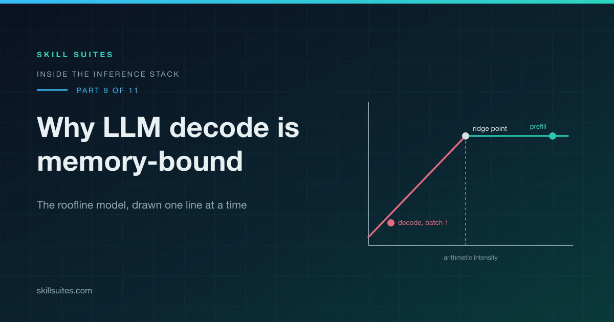
Both limits apply simultaneously. You cannot exceed the arithmetic rate and you cannot exceed the delivery rate. So the real ceiling at any intensity is whichever of the two is lower. On the left the diagonal is lower, so memory decides. On the right the flat line is lower, so compute decides. Keep only the lower value at every point and you get a rising slope that flattens into a ceiling. That is the profile of a pitched roof, and that is where the roofline model gets its name.
The corner where the two lines cross is the ridge point, the intensity at which the two limits are exactly balanced. It falls out of one division:
ridge point = peak FLOP/s / peak bytes/sFor an H100 SXM: 989 TFLOP/s divided by 3.35 TB/s is about 295 FLOPs per byte. Nothing about your model, your framework or your batch size appears in that calculation.
Definition
Ridge point
Peak FLOP/s divided by peak bytes/s, expressed in FLOPs per byte. It is the arithmetic intensity at which the diagonal meets the flat ceiling. For an H100 SXM, 989 TFLOP/s over 3.35 TB/s gives about 295 FLOPs per byte.
Origin: named in the 2009 roofline paper as the point where the two roofs meet, offered as a compact way to state how much data reuse a machine demands before it will run at full speed.
Why it matters: it is a pure hardware property, so you can compute it from a datasheet before you own the card. It is the single most useful number on a GPU spec sheet and no vendor prints it.
The ridge splits the plane in two
Drop a vertical line from the ridge and the chart divides into two territories. Left of the ridge, bytes arrive too slowly to keep the arithmetic units busy, so the tensor cores finish their work and wait. Right of the ridge, bytes arrive faster than the math can consume them, so the bus has slack.
Definition
Memory-bound and compute-bound
Two names for which wall you are pressed against. Below a ridge point of 295 the bus cannot deliver bytes fast enough to keep the tensor cores fed, so you are memory-bound. Above it the tensor cores cannot consume bytes as fast as they arrive, so you are compute-bound.
Origin: the vocabulary is older than the roofline model and was used loosely for decades. What the 2009 paper added was a way to compute which of the two you are, from one workload number and two hardware numbers, instead of arguing about it.
Why it matters: every optimisation targets one wall or the other. Widening the wall you are not touching costs real money and returns exactly zero.
Read the word “bound” literally. It means bounded by. It names the wall you are pressed against, and therefore the only wall worth attacking. Widening a corridor you are not standing in does nothing. That is the entire diagnostic value of the roofline model, and it is why the chart is worth twenty minutes of your time.
Section takeaways
- Both limits apply at once, so the ceiling at any intensity is the lower of the flat roof and the rising diagonal.
- The ridge point is peak FLOP/s over peak bytes/s. For an H100 SXM that is 989 divided by 3.35, about 295 FLOPs per byte.
- Nothing about your model, framework or batch size enters that division, so the ridge is a hardware constant you can read off a datasheet.
- Left of the ridge the tensor cores wait for bytes, which is memory-bound. Right of it the bus has slack, which is compute-bound.
- “Bound” means bounded by, so the label names the only wall worth attacking.
Where LLM work actually lands
The running example for this series is a Llama-3-70B class model: 80 layers, d_model of 8,192, roughly 70 billion parameters, held in bf16. That is about 140 GB of weights. If you want the model-side background on why the forward pass has the shape it does, Part 8 walks the original 2017 architecture box by box.
Definition
Prefill and decode
The two phases of a generation request. Prefill runs the whole prompt through the model once, all tokens together, and fills the KV cache. Decode then produces one token at a time, and every step reads all 140 GB of weights again to produce a single token.
Origin: the split is forced by autoregressive generation with a KV cache. The prompt is known up front and can be processed in parallel, while each generated token depends on the one before it. Pope and colleagues costed the two phases separately in 2022 and showed they sit in different performance regimes.
Why it matters: the two phases land on opposite sides of the ridge, so an intervention that transforms one of them can do nothing whatsoever for the other.
Two facts drive everything below. First, a forward pass does roughly 2 FLOPs per parameter per token (one multiply and one add). Second, a bf16 parameter occupies 2 bytes. Divide the first by the second and you get a rule you can carry around in your head:
The arithmetic intensity of a bf16 transformer step is approximately the number of tokens processed in that step.
One token in flight gives an intensity near 1. Thirty-two tokens gives roughly 32. Two thousand gives roughly 2,000. If you count fused multiply-add the way vendor spec sheets do, or you add the attention math on top, you get about twice those figures. The factor of two is not what matters here. The gap to the ridge is a factor of several hundred.
Definition
Matrix-vector versus matrix-matrix
Decode at batch 1 multiplies each weight matrix by a single vector, so every weight is read once and used once, giving an intensity near 1. Prefill and large batches multiply the same matrix by many vectors at once, so one weight read serves many multiply-adds and the intensity rises with the number of columns.
Origin: the distinction is baked into the BLAS interface. Matrix-vector operations became Level 2 in 1988 and matrix-matrix operations became Level 3 in 1990, and Level 3 exists specifically because only matrix-matrix work reuses data enough to hide the memory hierarchy.
Why it matters: batch size is the knob that turns a Level 2 shaped workload into a Level 3 shaped one. That is the whole mechanism behind batching.
Decode at batch 1
To produce one token, the model reads every weight in the network and does about 140 GFLOPs of math with them. Intensity lands at 1 to 2 FLOPs per byte, against a ridge of 295.
Multiply it out. Achieved performance is bandwidth times intensity: 3.35 TB/s times 1 gives 3.35 TFLOP/s, against a peak of 989 TFLOP/s. That is roughly one third of one percent of the chip’s arithmetic capacity. Be generous about the counting and call it one percent. Either way, more than 99 percent of the tensor cores you paid for are idle, and they are idle for the entire duration of every token you generate.
Analogy
Driving a 40 tonne lorry across the country to collect one screw, then driving back. The journey is the 140 GB weight read and the screw is the single token it produces.
Where it breaks: for one screw you could send a van. There is no smaller vehicle here, because producing even one token requires every weight in the network, so the only saving available is putting more screws on the same lorry.
The ceiling bandwidth alone imposes
Because the bytes are the bottleneck, you can compute a hard tokens-per-second ceiling without knowing anything about the software:
max tokens/sec = aggregate memory bandwidth / bytes of weights read per token140 GB does not fit on one 80 GB H100, so shard it across two with tensor parallelism. Each card now reads its own 70 GB shard per step. At 3.35 TB/s that takes 70 / 3350 = 20.9 ms. Both cards do it at the same time, so a decode step costs about 21 ms and you get roughly 48 tokens per second at batch 1.
Definition
Tensor parallelism
Splitting each weight matrix across several GPUs so every card holds a slice and every card does part of every matmul. Two H100s holding a 140 GB model each read a 70 GB shard per decode step, at the same time, then exchange partial results.
Origin: introduced for transformers by Shoeybi and colleagues in the 2019 Megatron-LM work, adopted because the largest models had outgrown the memory of any single device.
Why it matters: it divides the bytes each card must read, so it divides the decode step time, at the price of a collective communication on every step.
That number is an upper bound. No kernel, no compiler, no framework can beat it while the weights stay in bf16 and every one of them has to be read. Real systems land below it, because collective communication between the two cards and reads from the KV cache both add bytes. If your vendor demo shows 40 tokens per second on this setup, they are running at 83 percent of a physical limit and doing well. If a proposal promises 200, ask which of the four assumptions they broke.
In practice
Work the bandwidth-implied ceiling out before any vendor call: aggregate memory bandwidth divided by bytes of weights read per token. Two H100 SXM cards holding a 140 GB model give 6.7 TB/s against 140 GB, which is about 48 tokens per second at batch 1. If a quote promises three times that figure, ask which assumption moved: the precision, the parameter count, the batch size or the bandwidth. It is always one of those four.
Decode at batch 32
Run 32 sequences concurrently and the model reads the same 140 GB, once, and uses it to produce 32 tokens. The bytes did not increase. The math did, by 32 times.
Intensity moves from about 1 to about 32. The point slides right along the diagonal and up the roof. Throughput goes from 48 tokens per second to roughly 1,530. And the wall-clock time per step barely moves, because the step was always waiting on memory and memory is doing the same amount of work. Each individual user still sees a token roughly every 21 ms.
Thirty-two times the throughput for close to zero added latency. That is not a software trick. It is what the geometry of the chart says has to happen.
Prefill
Now process a 2,048 token prompt. Same weights, same 140 GB read, but every weight is used for 2,048 tokens at once. Total math is 2 x 70e9 x 2048, about 287 TFLOPs. Intensity is 287e12 / 140e9, roughly 2,048 FLOPs per byte, which is what the rule of thumb predicted.
That is seven times past the ridge. Prefill sits flat against the compute ceiling with the memory bus half asleep. This is the whole prefill and decode asymmetry, and it is why serving stacks increasingly run the two phases on separate machines with separate hardware. It is also why time-to-first-token and inter-token latency respond to completely different interventions, which matters a great deal if you are streaming responses and optimising perceived latency.
| Workload | Bytes read per step | FLOPs per step | Intensity | Relative to ridge (295) | Bounded by |
|---|---|---|---|---|---|
| Decode, batch 1 | ~140 GB | ~0.14 TFLOP | ~1 to 2 | 200x to the left | Memory bandwidth |
| Decode, batch 32 | ~140 GB | ~4.5 TFLOP | ~32 to 64 | Still left of it | Memory bandwidth |
| Prefill, 2,048 tokens | ~140 GB | ~287 TFLOP | ~2,048 | 7x to the right | Arithmetic rate |
Section takeaways
- A bf16 transformer step has an arithmetic intensity roughly equal to the number of tokens in that step, because 2 FLOPs per parameter divided by 2 bytes per parameter is 1.
- Decode at batch 1 sits at 1 to 2 FLOPs per byte against a ridge of 295, achieving about 3.35 TFLOP/s out of 989, under one percent of the chip.
- Two H100s reading a 70 GB shard each at 3.35 TB/s take 20.9 ms per decode step, capping batch-1 output at roughly 48 tokens per second.
- Batch 32 reads the same 140 GB and produces 32 tokens, moving intensity to about 32 and throughput to roughly 1,530, with per-user latency still near 21 ms.
- A 2,048 token prefill does about 287 TFLOPs on that same 140 GB read, an intensity near 2,048, which is seven times past the ridge.
The free lunch, and exactly where it ends
Every step rightward along the diagonal is throughput you get for almost no additional wall-clock time, because the bytes were already moving. Nobody is paying for it. That is a genuinely free lunch and it is the reason continuous batching exists.
Analogy
A bus already running its route. The eleventh passenger costs the operator nothing in fuel and nothing in time, which is exactly what happens when you add a sequence to a batch that is already waiting on memory.
Where it breaks: a bus has a fixed number of seats and refuses passengers at a single hard limit. Here there are two different limits at two different numbers: the ridge at roughly 150 to 300 sequences, and the KV cache running out of room, which usually arrives first.
The lunch stops at the ridge. Precisely there, and not one intensity unit further. Past the ridge you are compute-bound, the step time now scales with the amount of math, and adding another sequence to the batch buys you queueing delay and nothing else. On an H100 with a bf16 70B model, the ridge sits at a batch of roughly 150 to 300 concurrent sequences depending on how you count FLOPs, so from batch 1 you have a few hundred sequences of headroom to spend.
Two caveats keep this honest. Batching amortises weight reads and does not amortise KV cache reads, because every sequence carries its own KV cache and no two sequences share one. So as batch size and context length grow, KV traffic becomes the dominant memory cost, and the attention operation stays memory-bound no matter how large the batch gets.
The second caveat is why nobody actually reaches batch 300: you run out of memory to hold those KV caches long before you get there, and naive allocation wastes most of what is left. Part 10 covers continuous batching and PagedAttention, which is the story of what stops you from batching and what vLLM does about it.
Section takeaways
- Every step rightward along the diagonal is throughput bought with bytes that were already moving, so it costs almost no wall-clock time.
- The free lunch ends exactly at the ridge, which for a bf16 70B model on an H100 is a batch of roughly 150 to 300 sequences.
- Past the ridge, step time scales with the math, so extra batch buys queueing delay and no extra throughput.
- Batching amortises weight reads and never amortises KV cache reads, since no two sequences share a cache, so attention stays memory-bound at any batch size.
- KV cache memory, not the ridge, is what caps batch size in practice.
Three moves, and no others
Once a workload is placed on the roofline model, the set of things that can possibly help becomes finite and visible. There are three directions, and nothing else moves your point upward.
- Lift the diagonal. More memory bandwidth. Helps everything left of the ridge, proportionally.
- Slide right. Fewer bytes for the same math, or more math per byte. Helps until you hit the ridge.
- Raise the ceiling. More arithmetic capacity. Helps nothing left of the ridge.
Where the real techniques land
Almost every inference optimisation you have heard of is move 2, and almost all of them work by moving fewer bytes. The mechanisms are not interchangeable, so it is worth being exact about each one.
- Batching. More math per byte. FLOPs rise with batch size while bytes stay fixed, so the point slides right. This is the only one of the four that leaves bytes-per-step alone.
- Quantization. Fewer bytes per weight. Weight-only int4 quantization cuts the bytes by four while leaving the FLOP count untouched (the values are expanded back out before the multiply). Intensity goes up four times and the tokens-per-second ceiling goes up four times. This is the single largest batch-1 decode win available, which is exactly what the chart predicts.
- Mixture of experts. Fewer bytes per token, because only the routed experts get read. It is worth being exact: at batch 1 an MoE layer cuts the math by the same factor it cuts the bytes, so the intensity barely moves. What improves is the numerator of the ceiling formula. Fewer bytes per token means more tokens per second from the same bus. At large batch the tokens scatter across experts and you end up reading most of the weights anyway, which is why MoE helps decode more than it helps prefill.
- Kernel fusion and FlashAttention. Fewer bytes, same math. An unfused attention writes the full score matrix out to HBM and reads it back. FlashAttention keeps it in SRAM and never materialises it. The FLOPs are unchanged (slightly higher, in fact, because of recomputation), the HBM traffic collapses, and intensity rises. It is a pure move 2 with no accuracy cost, which is rare.
In practice
For a latency-sensitive single-stream workload, try weight-only int4 before anything else. It cuts bytes read per token by four, which raises the token ceiling by four, and the chart says that is the largest single move available on the left of the ridge. Measure output quality on your own evaluation set afterwards, because it is the one item on that list which can change what the model says.
Speculative decoding is move 2 by a different route
Definition
Speculative decoding
A small draft model proposes k tokens cheaply, and the large model verifies all k in a single forward pass, because it can score the whole proposed sequence in parallel. That one pass reads the 140 GB of weights once and does k tokens of math with them, so its intensity is roughly k instead of 1.
Origin: introduced by Leviathan, Kalman and Matias in 2022, to cut the latency of a single stream without changing the distribution the model samples from.
Why it matters: every token the verifier accepts is a token you got without a separate weight read, which is the only way to buy speed for one user rather than for a crowd.
What it converts is k serial memory-bound steps into one wider step, and that is the crucial difference from batching. Batching raises aggregate throughput for many users while holding per-user latency flat. Speculative decoding raises throughput for a single stream, which is the one thing batching cannot do. It also burns extra FLOPs on rejected tokens, which is fine, because on the left of the ridge you had FLOPs to spare. The economics only work while the acceptance rate stays high; a draft model that gets rejected constantly costs you its own bandwidth for nothing.
Section takeaways
- Three moves exist: lift the diagonal with bandwidth, slide right with intensity, or raise the ceiling with arithmetic. The third does nothing left of the ridge.
- Batching raises FLOPs at fixed bytes. Quantization, MoE and FlashAttention all cut bytes at roughly fixed FLOPs.
- Weight-only int4 cuts bytes per weight by four and leaves the FLOP count alone, so it raises intensity and the token ceiling by four.
- FlashAttention keeps the score matrix in SRAM instead of writing it to HBM, so it slides right with no accuracy cost and slightly more arithmetic.
- Speculative decoding verifies
kproposed tokens per weight read, lifting intensity to roughlyk, and it is the only move here that speeds up a single stream.
The expensive mistake this prevents
The mistake is buying move 3 for a workload that lives in move 2’s territory. A chip with twice the FLOP rate and identical bandwidth changes nothing about batch-1 decode. Zero. The ceiling was never the surface you were touching. You will pay a hardware premium, run the benchmark, see the same tokens per second, and spend a fortnight blaming the framework. Ten minutes with the roofline model would have told you the answer before the quote was signed.
Here are real accelerators with the ridge point worked out. Treat these as vendor peak specifications for dense bf16 with no sparsity. Measured numbers typically land 10 to 20 percent below peak, which shifts the ridge slightly but never enough to matter to the argument.
| Accelerator | Memory bandwidth | Peak bf16 (dense) | Ridge point |
|---|---|---|---|
| NVIDIA L40S (48 GB) | 864 GB/s | 362 TFLOP/s | ~419 FLOPs/byte |
| NVIDIA A100 SXM (80 GB) | 2.04 TB/s | 312 TFLOP/s | ~153 FLOPs/byte |
| NVIDIA H100 SXM (80 GB) | 3.35 TB/s | 989 TFLOP/s | ~295 FLOPs/byte |
| NVIDIA H200 SXM (141 GB) | 4.8 TB/s | 989 TFLOP/s | ~206 FLOPs/byte |
| AMD MI300X (192 GB) | 5.3 TB/s | 1,307 TFLOP/s | ~247 FLOPs/byte |
Look at the first two rows together, because that comparison is worth money. The L40S has a higher peak bf16 FLOP rate than an A100 80GB. It also has 42 percent of the bandwidth. For batch-1 decode of a model that fits on both, the A100 is about 2.4 times faster, and the card with the better spec-sheet headline loses badly.
In practice
If your workload is chat-shaped, with modest concurrency and latency that users can feel, the number on the quote that governs your experience is GB/s. Sort your options by bandwidth per dollar and by whether the model fits without sharding. Sort by TFLOP/s only if you are prefill-heavy, doing bulk document processing, batch summarisation or offline evaluation, where you genuinely sit right of the ridge.
This is also the arithmetic that should sit at the front of any decision about moving LLM workloads on-prem. Before you compare the capital cost of a GPU node against per-token API pricing, compute the bandwidth-implied token ceiling for the model you intend to run at the concurrency you actually expect. Two numbers off a datasheet and one division will tell you whether the box can serve your traffic at all. It is a much cheaper thing to get wrong on a whiteboard than in a purchase order, and Part 11 turns that estimate into a measurement of your own hardware in an afternoon.
Before you buy anything at all, though, check the cheapest speedup on the list. If you are memory-bound at low batch, raising concurrency costs nothing but scheduler work, and the free lunch is real all the way to the ridge.
Section takeaways
- A chip with twice the FLOP rate and identical bandwidth changes batch-1 decode by nothing, because the compute ceiling was never the surface being touched.
- The L40S has a higher peak bf16 rate than an A100 80GB and 42 percent of its bandwidth, so the A100 is about 2.4 times faster on batch-1 decode.
- Ridge points on current accelerators run from about 153 FLOPs per byte on an A100 to about 419 on an L40S, and decode sits near 1 on every one of them.
- Buy bandwidth for chat-shaped traffic and arithmetic for bulk prefill. The bandwidth-implied token ceiling is two datasheet numbers and one division.
Key takeaways
- The roofline model needs two hardware numbers: peak FLOP/s and peak bytes/s. Their ratio is the ridge point, which is where the memory diagonal meets the compute ceiling.
- The memory roof rises because performance equals bandwidth times intensity, and that proportionality draws as a 45 degree line on log axes. A 45 degree line on this chart is a bandwidth.
- The arithmetic intensity of a bf16 transformer step is roughly the number of tokens in that step. Batch 1 decode sits near 1, against ridge points of 150 to 420 on current accelerators.
- Decode at batch 1 uses well under one percent of a modern GPU’s arithmetic capacity. Its tokens-per-second ceiling is memory bandwidth divided by bytes of weights, and no software can exceed it.
- Batching is close to free until the ridge, because the bytes were already moving. Past the ridge it buys only queueing delay.
- Batching, quantization, MoE, kernel fusion and FlashAttention all slide you rightward, and all of them work by moving fewer bytes. Speculative decoding does the same thing for a single stream by verifying several tokens per weight read.
- Doubling the FLOP rate does nothing for batch-1 decode. Buy bandwidth for chat, buy arithmetic for bulk prefill.
Frequently asked questions
Is LLM inference memory-bound or compute-bound?
Both, depending on the phase. Decode (generating tokens one at a time) is heavily memory-bound, with an arithmetic intensity near 1 FLOP per byte against GPU ridge points of 150 to 420. Prefill (processing the prompt) is compute-bound, because thousands of tokens share a single read of the weights.
What is the ridge point of a GPU?
The ridge point is peak FLOP/s divided by peak memory bandwidth, expressed in FLOPs per byte. It is the arithmetic intensity at which the two limits balance exactly, and it is a pure property of the hardware with no dependence on your model or framework. An H100 SXM sits near 295 FLOPs per byte.
How do I calculate the maximum tokens per second for a model on my GPU?
Divide your aggregate memory bandwidth by the bytes of weights read per token. A 70B model in bf16 is about 140 GB, so two H100 SXM cards at 3.35 TB/s each give roughly 48 tokens per second at batch 1. That is a hard upper bound that no serving software can beat.
Does a faster GPU make single-user LLM generation faster?
Only if the newer chip has more memory bandwidth. Batch-1 decode never touches the compute ceiling, so a card with twice the FLOP rate and the same bandwidth will produce identical tokens per second. Compare GB/s, not TFLOP/s, when latency for one user is what you care about.
Why does batching increase throughput without increasing latency?
Because the weight bytes were already being moved. At batch 1 the arithmetic units sit idle waiting for memory, so adding more sequences fills that idle time with useful math instead of extending the step. The effect holds until arithmetic intensity reaches the ridge point, after which extra batch adds queueing delay.
Does quantization help because of fewer FLOPs or fewer bytes?
Fewer bytes, in the decode case. Weight-only int4 quantization leaves the FLOP count essentially unchanged and cuts the bytes read per token by four, which raises both the arithmetic intensity and the bandwidth-implied token ceiling by the same factor. That is why it is the largest single win available for memory-bound decode.
Sources and further reading
- Roofline: An Insightful Visual Performance Model for Multicore Architectures, Williams, Waterman and Patterson, the original 2009 paper.
- Efficiently Scaling Transformer Inference, Pope et al., which works the arithmetic intensity of transformer inference through in detail.
- FlashAttention: Fast and Memory-Efficient Exact Attention with IO-Awareness, the canonical example of optimising an operation by cutting HBM traffic.
- Fast Inference from Transformers via Speculative Decoding, Leviathan, Kalman and Matias.
- Efficient Memory Management for Large Language Model Serving with PagedAttention, the vLLM paper.
- vLLM documentation, for the batching and scheduling behaviour discussed in Part 10.
Check your understanding
Take the 15 question quiz on this article
The same 15 questions every time, picked to cover every idea this article teaches, out of 30 written for it. The order of the questions and the order of the answer choices reshuffle on every attempt, so a retake never looks identical to the last one. It runs here on the page and keeps your place, so you can go and read a section and come back without losing anything. You get a full report at the end: your score, the correct answer to anything you missed, why it is correct, and a link straight back to the section it came from.
- 15 questions
- same set every time
- 8 knowledge areas
- hint on every question
- timed, no limit
