
How neural networks learn is one of those topics that gets explained backwards. Most guides open with a diagram of a hundred glowing circles wired together, drop the word “backpropagation,” and hope you nod along. This guide does the opposite. We start with a single number being multiplied by another number, and we do not add a new idea until the previous one is airtight. By the end you will have built a complete, working neural network in your head — and then in about 60 lines of plain Python that actually trains.
No prerequisites beyond arithmetic. No hand-waving. Every concept arrives with real numbers you can check on paper, and each one is the smallest possible step past the last. This is Part 1 of a from-scratch series: it takes you from one neuron all the way to backpropagation and a full training loop — the entire engine that every large model on Earth is built from.
- A neuron (multiply → sum → add bias → activate)
- A layer, then a stack of layers — the forward pass
- The loss: one number for “how wrong”
- The gradient, gradient descent, the chain rule, and backpropagation
- A runnable network that learns XOR from scratch — and a look at its decision boundary bending into shape as it trains
In a hurry? The diagrams carry the whole story on their own — the neuron, the forward pass, the training loop, the falling loss, and the decision boundary bending into shape. The prose is here for when you want the why.
Concept 1 — A neuron is just multiplication
Forget the biology. At its core, a single neuron takes one number coming in, multiplies it by its own private number called a weight, and passes the result out. That is the whole thing:

output = weight × input
Say the input is 2 and this neuron’s weight is 3. Then output = 3 × 2 = 6. The input is given to you — it’s the data. The weight belongs to the neuron; it’s the only thing the neuron “owns.” When people say a neural network learns, they mean it is adjusting these weights. Nothing else moves. The inputs are whatever they are; the weights are the knobs.
So a neuron is a knob that scales whatever flows through it. A weight bigger than 1 amplifies the input; between 0 and 1 it shrinks it; a weight of 0 kills it entirely; a negative weight flips its sign. That is concept one, and it never changes.
Concept 2 — Many inputs: the weighted sum
One input was a warm-up. Real neurons receive several numbers at once, and each input gets its own weight — its own knob. You multiply each input by its matching weight, then add the results into a single number.
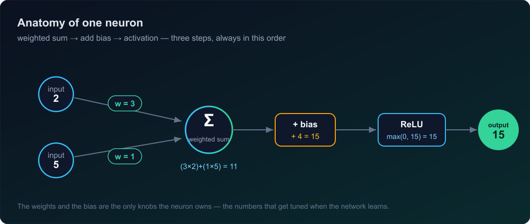
Two inputs come in, 2 and 5. The neuron has two weights, 3 and 1:
(3 × 2) + (1 × 5) = 6 + 5 = 11
Multiply in pairs, add the pile together, one number comes out. Why sum? Because the neuron has to collapse many inputs into a single output to pass forward. Addition is how it pools everything into one verdict, and each weight decides how loudly that input gets to vote. A weight of 0 means “I don’t care about this input,” and it drops out of the sum.
This pattern — multiply each input by a weight, then sum — is called a weighted sum. Burn that phrase in. It is the engine inside every neuron in every network ever built. A model with billions of parameters is doing exactly this, just billions of times.
Concept 3 — The bias: a baseline the inputs can’t touch
Now the neuron adds one more number that isn’t tied to any input. Say the bias is 4:
(3 × 2) + (1 × 5) + 4 = 11 + 4 = 15
The bias multiplies nothing. It just sits there and gets added every single time. Why bother? Because without it, if every input is 0 the output is forced to be 0 — the neuron has no choice. The bias breaks that. It lets the neuron hold a baseline, a default lean, even when the inputs say nothing:
(3 × 0) + (1 × 0) + 4 = 4
Think of the weighted sum as the evidence and the bias as the neuron’s prior opinion. A high positive bias means “I lean toward firing unless the evidence drags me down”; a negative bias means “I stay quiet unless the evidence pushes me hard enough.” And like the weights, the bias is a knob — a number the neuron owns and tunes when it learns. So a neuron’s tunable parts are exactly: one weight per input, plus one bias.
Concept 4 — The fatal flaw, and the fix that makes networks powerful
Here is a problem that sinks everything we have so far. Take a neuron that doubles its input (output = 2 × input) and feed its result into a second neuron that triples (output = 3 × input). Input 5 → first neuron → 10 → second neuron → 30. Two neurons, two layers — but 30 is just 6 × 5. You could have used a single neuron with weight 6 and gotten the identical answer. The two layers bought you nothing.
This always happens. Multiplying and adding, then multiplying and adding again, can always be rewritten as a single multiply-and-add. Stack a thousand layers of pure weighted sums and a mathematician can flatten the whole thing back into one. The depth is fake. A pile of weighted sums can only ever draw straight-line relationships — double the input, double the output, forever. It can never bend.
But the real world bends. “A little salt improves the soup; a lot ruins it.” More is not always proportionally better — that is a curve, not a line, and a stack of weighted sums physically cannot represent it.
The fix: after the neuron computes its number, pass it through a function that bends. The most common one is brutally simple. It is called ReLU (Rectified Linear Unit), and it is one rule: if the number is negative, output 0; if it’s positive, keep it.
ReLU(15) = 15 ReLU(−7) = 0 ReLU(3) = 3 ReLU(−0.2) = 0
That tiny kink is the bend. Because a neuron can now switch off (output 0) for some inputs and stay alive for others, stacking neurons stops collapsing — each one handles its own slice of the situation and the layers no longer flatten into one. That little corner at zero is the whole reason deep networks can model curves, edges, and anything that isn’t a straight line. (ReLU is the default today because it’s cheap and trains well; sigmoid and tanh are older alternatives with the same job.)
So the complete neuron is three steps, always in this order:
Concept 5 — A layer: neurons side by side
So far we have watched one neuron. Now put three in a row. They all receive the same inputs — but each owns a different set of weights and its own bias, so each produces a different number. Feed the same pair (2, 5) into all three:
| Neuron | Weights & bias | Weighted sum + bias | After ReLU |
|---|---|---|---|
| A | (3, 1), b=4 | (3×2)+(1×5)+4 = 15 | 15 (screaming) |
| B | (−2, 1), b=0 | (−2×2)+(1×5)+0 = 1 | 1 (whispering) |
| C | (1, −3), b=2 | (1×2)+(−3×5)+2 = −11 | 0 (silent) |
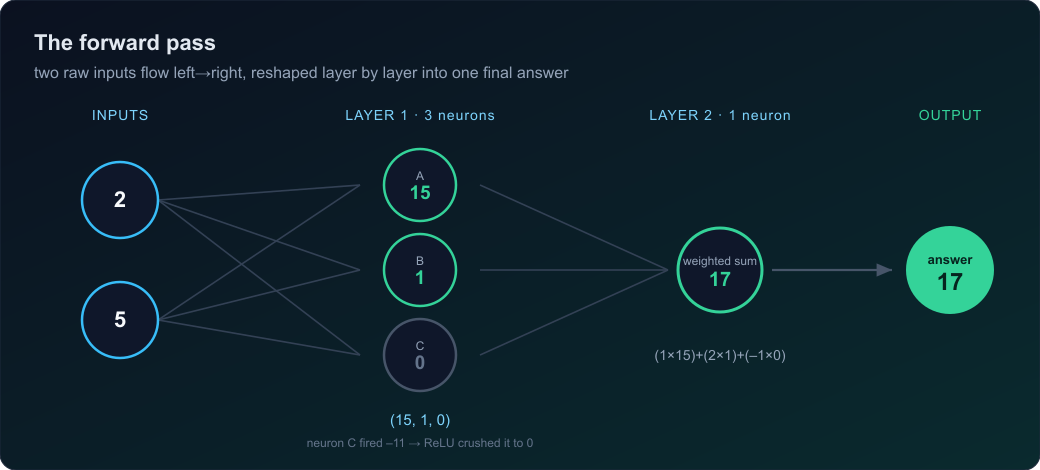
Two numbers went in; three came out: (15, 1, 0). That is a layer. Notice what happened to the shape: the number of neurons in a layer decides how many numbers come out the other side — nothing else. And look at neuron C: it computed −11, then ReLU crushed it to 0. It switched off for this particular input. Same inputs, three different reactions — each neuron has quietly become a specialist, tuned by its own weights to care about a different pattern.
Here is the move that makes everything click: those three outputs are themselves just numbers, which means they can become the inputs to another layer. Feed (15, 1, 0) into a fresh row of neurons and you have stacked layers — a deep network.
Concept 6 — The forward pass
Take our layer’s output (15, 1, 0) and feed it into a second layer. Let’s make this one a single neuron, because we want the network to end on one final number — a verdict. Its three weights (one per incoming number) are (1, 2, −1), bias 0:
(1×15) + (2×1) + (−1×0) + 0 = 17 → ReLU → 17
Trace the whole journey: (2, 5) → Layer 1 → (15, 1, 0) → Layer 2 → 17. Two raw inputs walked in, got reshaped into three specialist signals, then those got pooled into one final number. That entire left-to-right journey — inputs entering, flowing through each layer, emerging as an output — is the forward pass. “Forward” because data moves one direction only: in the front, out the back. Multiply, sum, bias, activate — repeat per layer — until a number falls out the end.
Now sit with the most important realization so far. Every weight and bias in that journey was a number we made up. So 17 is almost certainly wrong. The network ran its machinery flawlessly and produced a confidently incorrect answer, because its knobs are set to random junk. That is not a bug — it is the starting condition of every neural network before training. A fresh network is a perfectly functioning machine full of random knobs, producing garbage on purpose. Which forces the real question: how wrong is 17? Not “is it wrong,” but by how much, as a single hard number we can chase toward zero.
Concept 7 — The loss: one number for “how wrong”
The network said 17. Suppose the correct answer — the real house price, the true score — was 20. We know it because this is training data: examples where the right answer is written down. That right answer is called the target (or label). So we have two numbers: what the network said (17) and what it should have said (20). The loss turns the gap between them into a single score. The simplest way is to take the difference and square it:
error = 17 − 20 = −3 loss = (−3)² = 9
Why square it? Two reasons, both practical. First, it kills the minus sign: guessing 23 gives error +3, equally wrong in the other direction, and squaring makes both come out to 9. We care how far the miss was, not which way. Second, squaring punishes big misses harder — off by 3 → loss 9; off by 10 → loss 100; off by 30 → loss 900. A badly broken prediction screams; a near-miss barely whispers. (This is mean squared error, the standard loss for predicting numbers; classification tasks use a cousin called cross-entropy.)
So the loss is the network’s report card compressed to one number: big loss = very wrong, zero loss = perfect. And now the entire purpose of training snaps into focus. Learning = changing the weights and biases until the loss gets as close to zero as possible. That is the whole game. Every neural network ever trained is a hunt to shrink one number. Which leaves exactly one question, and it is the question: we have loss 9 and a pile of knobs — which knob do we turn, and in which direction, to make 9 smaller?
Concept 8 — The gradient: measure, don’t guess
Don’t guess which way to turn a knob — measure it. Pick one weight, give it a tiny nudge, and watch what the loss does. Our final neuron had weights (1, 2, −1) reading inputs (15, 1, 0), giving 17, target 20, loss 9. Interrogate the first weight, currently 1. Nudge it up a hair, from 1 to 1.1, and rerun the forward pass:
(1.1×15) + (2×1) + (−1×0) = 18.5 loss = (18.5 − 20)² = 2.25
The loss fell from 9 to 2.25 just because we pushed that one weight up slightly. Turn that into a number:
(2.25 − 9) ÷ 0.1 = −67.5
That ratio, −67.5, is the gradient of the loss with respect to that weight. It answers a precise question: per unit of change in this weight, how does the loss move? Two things it tells you, and they are everything:
- Direction. The gradient is negative, so weight-up → loss-down. To shrink the loss, push this weight up. A positive gradient means the opposite. The rule is dead simple: move the knob opposite to the sign of its gradient.
- Magnitude. −67.5 is big — this weight has enormous leverage over the loss. A weight with gradient −0.3 barely matters. So the gradient also tells you which knobs are worth turning.
That is the gradient: for each knob, one number saying which way to turn it and how much it matters.
Nudging by 0.1 and dividing is a finite approximation. Calculus gives the exact slope by shrinking the nudge toward zero, and for our two pieces the rule is short. The loss is L = (out − target)², whose exact sensitivity to the output is its derivative dL/d(out) = 2×(out − target) = 2×(17 − 20) = −6. The output is out = w×15 + …, so its sensitivity to our weight is simply the input that weight multiplies, d(out)/dw = 15. Multiply the two — that is the chain rule, arriving in Concept 10 — to get the exact gradient: dL/dw = −6 × 15 = −90. Our finite nudge estimated −67.5; the gap exists only because a step of 0.1 is not infinitely small (squared loss curves sharply). Shrink the nudge to 0.001 and the estimate becomes −89.8, sliding straight toward the exact −90. Same idea, sharper tool — and notice the exact rule 2×(out − target) is exactly the “blame” number backpropagation will start from.
Concept 9 — Gradient descent: walking the loss downhill
We measured one knob’s gradient: −67.5. Here is what you actually do with it — the update rule, in one line:
new weight = old weight − (learning rate × gradient)
There’s a new character here, the learning rate — a small number you choose that controls how big a step to take. Use 0.001:
new weight = 1 − (0.001 × −67.5) = 1 + 0.0675 = 1.0675
Watch the signs do the work. The gradient was negative, so subtracting it added to the weight — exactly the direction that lowers the loss. You never decide “up or down” yourself; the minus sign in the rule plus the sign of the gradient sort it out every time. Why not take the full step? Because the gradient is only trustworthy for a tiny neighborhood — −67.5 describes the slope right here, not a mile away. Leap too far and you overshoot the bottom and the loss can shoot up.
| Learning rate | What happens |
|---|---|
| Too big (e.g. 1.0) | Giant lurching steps overshoot the minimum; loss bounces or explodes. |
| Too small (e.g. 0.0000001) | Creeps toward the answer so slowly training takes forever. |
| Just right | Big enough to make progress, small enough not to overshoot. |
The name pictures it perfectly: you’re standing on a hillside (the loss), the gradient points downhill, and you descend one careful step at a time toward the valley where the loss is smallest. That is gradient descent. But we cheated: to get that gradient we brute-forced it — nudge the weight, rerun the whole forward pass, measure. Fine for one knob. A real network has billions. Re-running the entire network billions of times per step is impossibly slow. So there has to be a clever way to get all the gradients at once, cheaply, in a single sweep. There is.
Concept 10 — The chain rule: effects multiply along a path
This is the one idea that makes the clever way possible. Use the cleanest example: one weight w = 2, one input x = 3, no bias, no activation. Two steps:
z = w × x = 6 loss = (z − target)², target 4 → (6 − 4)² = 4
We want the gradient of the loss with respect to w. Notice w doesn’t touch the loss directly — it touches z, and z touches the loss. Two links in a chain: w → z → loss. Measure each link separately:
- Link 1 — how much does z change when w changes?
z = w × 3, so nudgingwup by 1 moveszby 3. Local effect: 3 (it’s just the inputx). - Link 2 — how much does the loss change when z changes? At
z = 6the error is 2, and the loss moves by about 4 per unit ofz. Local effect: 4.
The chain rule says: just multiply the links.
gradient of loss w.r.t. w = 3 × 4 = 12
The effect of w on the loss is the effect of w on z, times the effect of z on the loss. Effects multiply along the chain. Check by brute force: nudge w from 2 to 2.1, then z = 6.3, loss = (2.3)² = 5.29, change 1.29 over 0.1 → ≈ 12.9. The chain rule said 12; they agree (the gap is the finite-nudge approximation again).
Sit with why this is the whole game. Each link is local — it depends only on the one little operation right there. Compute each link once, cheaply, looking only at its own step; then multiply links to get any knob’s gradient, no matter how far it sits from the loss. A knob ten layers deep? Its gradient is ten local effects multiplied down the chain. And you compute them starting at the loss and multiplying backward toward the knob — which is exactly where the next concept gets its name.
Concept 11 — Backpropagation: one backward sweep for every gradient
Now watch the chain fan out across a whole network, and watch the reuse that makes it cheap. Here is a network small enough to trace by hand. First the forward pass:
hidden A: weight a = 3 → 3×2 = 6 → ReLU → h_A = 6
hidden B: weight b = 1 → 1×2 = 2 → ReLU → h_B = 2
output: weights p = 1 (on h_A), q = 2 (on h_B) → (1×6)+(2×2) = 10
target = 6 → loss = (10 − 6)² = 16
Four knobs need gradients: p, q, a, b. Now the backward sweep — start at the loss and carry one number backward.
- Blame at the output. How does loss move per unit of the output?
loss = (out − 6)², local effect= 2×(out − 6) = 2×4 = 8. Call this8the output neuron’s blame signal. Everything reuses it. - Output-weight gradients = blame × the input that weight multiplied:
p: 8×6 = 48q: 8×2 = 16. Both built from the same 8 — that’s the reuse. - Push blame backward to the hidden neurons, scaled by the connecting weight:
blame→A = 8×p = 8blame→B = 8×q = 16. (Both pre-activations were positive, so ReLU’s local effect is 1 and the blame passes through unchanged.) - Hidden-weight gradients = blame × the input it multiplied (here x = 2):
a: 8×2 = 16b: 16×2 = 32.
Done. One sweep, four gradients — p:48, q:16, a:16, b:32 — and we never re-ran the forward pass. Quick brute-force check on p: nudge it from 1 to 1.1, new out = 10.6, new loss = (4.6)² = 21.16, change 5.16 over 0.1 → ≈ 51.6. Backprop said 48; they agree. That is backpropagation, stated plainly:
Each neuron computes one blame number — how much the loss cares about it — then (a) hands each of its weights a gradient = blame × that weight’s input, and (b) passes blame further back to the neurons feeding it, scaled by the connecting weights. Every neuron does this identical local job. Blame flows from the loss at the output, splitting and fanning backward, until every knob in every layer has its gradient.
That is why a network with billions of weights is trainable at all: the cost is just one forward pass and one backward pass per step, no matter how many knobs. This backward sweep — the gradient of the loss propagated back through the network — is the single most important algorithm in the field, introduced for neural nets in a 1986 paper by Rumelhart, Hinton, and Williams.
The full training loop, assembled
Every concept above snaps into a single loop. This loop is a neural network learning — the whole thing:
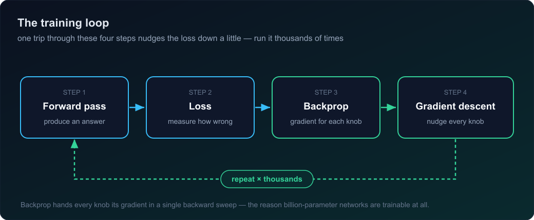
- Forward pass — inputs flow through, producing an answer.
- Loss — measure how wrong it is.
- Backpropagation — one backward sweep hands every knob its gradient.
- Gradient descent — nudge every knob opposite its gradient.
- Repeat thousands of times — the loss slides downhill and the answers stop being garbage.
Now run it: a neural network from scratch, in pure Python
Enough paper. Here is the entire loop as a real program — no libraries, just the arithmetic above. It learns XOR: output 1 when the two inputs differ, else 0. XOR is the classic problem no straight line can separate, so it only becomes solvable because of the hidden layer and the ReLU nonlinearity from Concept 4. The network is 2 inputs → 8 hidden neurons (ReLU) → 1 output.
import random
random.seed(7)

# XOR: output is 1 when the two inputs differ, else 0.
DATA = [((0.,0.),0.), ((0.,1.),1.), ((1.,0.),1.), ((1.,1.),0.)]
N_IN, N_HID, LR = 2, 8, 0.1

rnd = lambda: random.uniform(-1., 1.)          # small random starting weight
W1 = [[rnd() for _ in range(N_IN)] for _ in range(N_HID)]  # hidden weights
b1 = [rnd() for _ in range(N_HID)]                         # hidden biases
W2 = [rnd() for _ in range(N_HID)]                         # output weights
b2 = rnd()                                                 # output bias

relu = lambda z: z if z > 0 else 0.

def forward(x):
    pre = [sum(W1[j][i]*x[i] for i in range(N_IN)) + b1[j] for j in range(N_HID)]
    h   = [relu(z) for z in pre]               # hidden activations
    out = sum(W2[j]*h[j] for j in range(N_HID)) + b2   # output neuron
    return pre, h, out

for epoch in range(3001):
    loss = 0.
    for x, target in DATA:
        pre, h, out = forward(x)
        loss += (out - target) ** 2            # squared-error loss
        d_out = 2. * (out - target)            # blame at the output
        # push blame back FIRST, using output weights as they were this pass
        blame = [d_out*W2[j] if pre[j] > 0 else 0. for j in range(N_HID)]
        for j in range(N_HID):                 # update output knobs
            W2[j] -= LR * d_out * h[j]
        b2 -= LR * d_out
        for j in range(N_HID):                 # update hidden knobs
            if blame[j] == 0.: continue
            for i in range(N_IN):
                W1[j][i] -= LR * blame[j] * x[i]
            b1[j] -= LR * blame[j]
    if epoch in (0,20,40,60,80,100,500,1500,3000):
        print(f"epoch {epoch:>4}  loss {loss:.4f}")

print("\nlearned predictions:")
for x, target in DATA:
    print(f"  {x} -> {forward(x)[2]:+.3f}   (target {target})")
Save it as nn.py and run python nn.py (any Python 3 — no pip install needed). You’ll watch the loss slide downhill and the four predictions lock onto XOR:
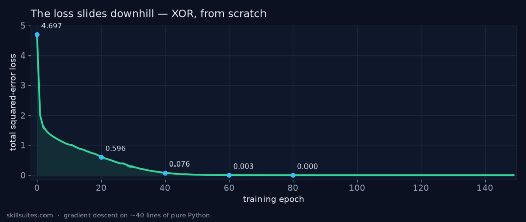
epoch    0  loss 4.6972
epoch   20  loss 0.5956
epoch   40  loss 0.0763
epoch   60  loss 0.0026
epoch   80  loss 0.0000
epoch 3000  loss 0.0000

learned predictions:
  (0.0, 0.0) -> -0.000   (target 0.0)
  (0.0, 1.0) -> +1.000   (target 1.0)
  (1.0, 0.0) -> +1.000   (target 1.0)
  (1.0, 1.0) -> +0.000   (target 0.0)
Those numbers are the loss walking downhill — the same descent from Concept 9, now happening for real. Plotted, the slide is unmistakable:
That is it. Every idea in this article — weighted sum, bias, ReLU, forward pass, squared-error loss, the “blame” sweep of backprop, and the gradient-descent update — is in those ~40 lines, and together they make a machine that starts out guessing garbage and teaches itself a function no single line could ever draw. (We use squared-error loss here so every line traces back to the concepts above; XOR is technically classification, where you’d normally reach for cross-entropy, but plain MSE trains it cleanly and adds no new machinery.) Prefer a prebuilt tool later? This is exactly what PyTorch and TensorFlow automate — they compute these gradients for you, on a GPU, for billions of parameters. But the loop is this loop.
The four checks above are the same four examples the network trained on. For XOR that is fair — those four cases are the entire input space, so there is nothing unseen to generalize to. But in almost every real problem you deliberately hold out a test set the network never trains on, because the goal is to generalize, not memorize. A model that scores perfectly on its training data yet fails on new data hasn’t learned — it has overfit, the central hazard of machine learning, and a topic we take up later in this series.
Watch the decision boundary bend
Numbers falling is one thing; seeing what the network learned is another. Because XOR has only two inputs, we can colour in the network’s answer for every point in the unit square and watch its decision boundary — the line where it flips from “0” to “1” — take shape as training runs. Below, the white line is that boundary; the sky and emerald basins are the two answers.
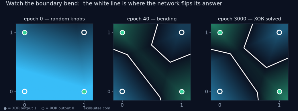
At epoch 0 the knobs are random: the surface is a smooth ramp and the network gives essentially the same answer everywhere — useless, exactly as promised. By epoch 40 the boundary is visibly bending as gradient descent carves the two emerald basins toward the corners that should output 1. By epoch 3000 it has wrapped into the only shape that solves XOR: opposite corners share an answer, and the boundary curves between them. No straight line can do that — and that bent boundary is precisely what the ReLU nonlinearity from Concept 4 buys you. Strip the activation out and this picture can only ever be a single straight cut, and XOR stays unsolvable forever. This is the whole argument of Concept 4, now something you can see.
ReLU neurons can “die.” If a neuron’s weighted sum is negative for every training example, ReLU outputs 0, its local gradient is 0, and it never updates again — a permanently dead knob. With too few hidden neurons, an unlucky random start can leave too few alive to bend the boundary, and gradient descent settles into a shallow local minimum (on XOR that shows up as loss stuck around 0.7). The fixes are exactly what real training uses: more hidden neurons (we use 8 for margin), a different random seed, or smarter weight initialization. It’s an honest first taste of why width and initialization matter — topics that return later in this series.
Where this goes next
You now own the complete learning engine. Everything else in deep learning is variations and scaling of exactly this loop. Upcoming parts of this from-scratch series build outward from here:
- Part 2 — Vectors & matrices: our scalars turn into arrays, and the layer becomes a single matrix multiply — the step that lets a network process thousands of inputs at once and run on a GPU.
- Later parts: softmax and cross-entropy for classification, better optimizers (momentum, Adam), regularization and overfitting, and the leap to convolutions and attention.
If your interest is less “build the math” and more “ship the model,” two companion reads pick up where the theory ends: why AI demos die in production, and the on-prem vs. hosted LLM decision — because once you understand what a model is, the hard part becomes running it. For the wider skill map, see the skills to learn in 2026.
- A neuron does three things, always in order: weighted sum → add bias → activation. Weights and biases are the only knobs it owns.
- Without a nonlinearity like ReLU, stacked layers collapse into one — depth is fake. The bend is what makes depth real.
- The forward pass turns inputs into an answer; the loss turns the error into one number to minimize.
- The gradient measures each knob’s effect on the loss; gradient descent nudges every knob opposite its gradient.
- Backpropagation computes all gradients in one backward sweep of “blame” — the reason billion-parameter models are trainable.
- Training is just this loop repeated thousands of times: forward → loss → backprop → descent.
Frequently asked questions
What’s the difference between a weight and a bias?
A weight multiplies an input — it decides how loudly that input votes in the neuron’s weighted sum. A bias multiplies nothing; it is a constant added at the end that gives the neuron a baseline, so it can produce a non-zero output even when every input is 0. Both are tunable knobs adjusted during training.
Why do neural networks need an activation function?
Without a nonlinear activation, every layer is just a weighted sum, and stacking weighted sums always collapses mathematically into a single weighted sum — so extra layers add no power and the network can only model straight-line relationships. A nonlinearity like ReLU introduces a bend, letting neurons switch on and off so deep networks can represent curves and complex patterns.
What exactly is backpropagation?
Backpropagation is an efficient algorithm for computing the gradient of the loss with respect to every weight and bias in one backward sweep. Each neuron computes a single “blame” number (how much the loss cares about it), hands each of its weights a gradient of blame × input, and passes blame further back through the connecting weights. It relies on the chain rule and costs just one forward pass plus one backward pass per step.
What is the learning rate, and how do I choose it?
The learning rate is a small number that scales each update step in gradient descent (new = old − learning_rate × gradient). Too large and training overshoots and diverges; too small and it converges painfully slowly. Common starting values are around 0.1 to 0.001, tuned by watching whether the loss falls smoothly.
Do I need calculus to understand how neural networks learn?
No. The core intuition — nudge a knob, see how the loss changes, move opposite the change — needs only arithmetic, which is how this guide builds it. Calculus simply gives the exact gradient (an infinitely small nudge) instead of the finite approximation, and libraries like PyTorch compute it for you automatically.
Can a neural network really learn from just this loop?
Yes. The runnable example above trains a from-scratch network to solve XOR — a problem no straight line can separate — using only a forward pass, a squared-error loss, backpropagation, and gradient descent. Every large model is the same loop scaled up with more layers, more data, and hardware acceleration.
Why did my neural network get stuck at a high loss?
A common cause is “dead” ReLU neurons: if a neuron’s weighted sum is negative for every training example, ReLU outputs 0, its gradient is 0, and it stops updating. With too few hidden neurons an unlucky random start can leave too few alive to learn the pattern, and gradient descent settles into a shallow local minimum — on XOR that often looks like a loss stuck around 0.7. Fixes are more hidden neurons, a different random seed, better weight initialization, or a smaller learning rate.
Educational walkthrough. The numbers and code are deliberately tiny so every step is checkable by hand; production networks use vectorized math, more sophisticated optimizers, and far more data, but the underlying loop is identical. Further reading: 3Blue1Brown’s neural network series, Michael Nielsen’s free book, and the Stanford CS231n backprop notes.
